Code
# Paths
library(here)

# Multivariate analysis
library(ade4)
library(adegraphics)

# Matrix algebra
library(expm)

# Plots
library(CAnetwork)# Paths
library(here)
# Multivariate analysis
library(ade4)
library(adegraphics)
# Matrix algebra
library(expm)
# Plots
library(CAnetwork)This is an extension of reciprocal scaling defined for correspondence analysis by Thioulouse and Chessel (1992) to double-constrained correspondence analysis.
Here, we have 3 matrices:
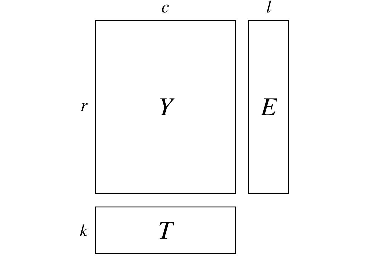
(r <- dim(Y)[1])[1] 26(c <- dim(Y)[2])[1] 21(l <- ncol(E))[1] 6(k <- ncol(T_))[1] 7# Define bound for comparison to zero
zero <- 10e-10We compute the \(H_k(i, j)\) from the LC scores computed with dcCA (noted \(LC\) for rows LS scores and \(CC\) for columns LC scores). This formula is a direct extension of formula (11) in Thioulouse and Chessel (1992) but we replace the ordination scores obtained with CA with the ordination scores obtained with dcCA.
\[ H_k(i, j) = \frac{LC_k(i) + CC_k(j)}{\sqrt{2 \lambda_k \mu_k}} \]
Ydf <- as.data.frame(Y)
ca <- dudi.coa(Ydf,
               scannf = FALSE,
               nf = min(r - 1, c - 1))

neig <- min(c(k, l))
dcca <- dpcaiv2(dudi = ca,
                dfR = E,
                dfQ = T_,
                scannf = FALSE,
                nf = neig)

L_dcca <- dcca$li
C_dcca <- dcca$co

lambda_dcca <- dcca$eig
mu_dcca <- 1 + sqrt(lambda_dcca)
# Transform matrix to count table
Yfreq <- as.data.frame(as.table(Y))
colnames(Yfreq) <- c("row", "col", "Freq")
# Remove the cells with no observation
Yfreq0 <- Yfreq[-which(Yfreq$Freq == 0),]
Yfreq0$colind <- match(Yfreq0$col, colnames(Y)) # match index and species names
# Initialize results matrix
H <- matrix(nrow = nrow(Yfreq0),
ncol = length(lambda_dcca))
for (kl in 1:length(lambda_dcca)) { # For each axis
ind <- 1 # initialize row index
for (obs in 1:nrow(Yfreq0)) { # For each observation
i <- Yfreq0$row[obs]
j <- Yfreq0$col[obs]
H[ind, kl] <- (L_dcca[i, kl] + C_dcca[j, kl])/sqrt(2*lambda_dcca[kl]*mu_dcca[kl])
ind <- ind + 1
}
}To perform the canonical correlation analysis, we compute the inflated tables \(R\) (\(\omega \times l\)) and \(C\) (\(\omega \times k\)) from \(E\) (\(r \times l\)) and \(T\) (\(r \times k\)). \(R\) and \(C\) are respectively equivalents to \(E\) and \(T\) where rows of are duplicated as many times as there are correspondences in \(Y\).
We take the frequency table defined before and use it to compute the inflated tables (with weights):
# Create indicator tables
tabR <- acm.disjonctif(as.data.frame(Yfreq0$row))
tabR <- as.matrix(tabR) %*% as.matrix(E)
tabC <- acm.disjonctif(as.data.frame(Yfreq0$col))
tabC <- as.matrix(tabC) %*% as.matrix(T_)

# Get weights
wt <- Yfreq0$Freq
Below are the first lines of tables \(R\) and \(C\):
| location | elevation | patch_area | perc_forests | perc_grasslands | ShannonLandscapeDiv |
|---|---|---|---|---|---|
| 0 | 10 | 6.28 | 7.7882 | 67.7785 | 0.232 |
| 0 | 30 | 7.92 | 16.4129 | 43.4066 | 0.274 |
| 0 | 430 | 83.24 | 24.4526 | 28.4995 | 0.274 |
| 0 | 420 | 140.83 | 41.9966 | 34.2412 | 0.260 |
| 0 | 400 | 140.83 | 41.9966 | 34.2412 | 0.260 |
| 0 | 500 | 0.50 | 7.5445 | 67.0780 | 0.240 |
| 0 | 470 | 7.84 | 19.3087 | 56.4031 | 0.253 |
| 0 | 110 | 21.15 | 23.4668 | 49.8908 | 0.262 |
| 0 | 460 | 24.82 | 21.3932 | 57.0430 | 0.243 |
| 0 | 450 | 3.11 | 4.8285 | 73.7518 | 0.216 |
| 0 | 40 | 6.66 | 7.4729 | 66.0061 | 0.240 |
| 0 | 160 | 5.63 | 32.3516 | 45.0477 | 0.253 |
| 0 | 160 | 10.99 | 29.7139 | 18.8270 | 0.291 |
| 1 | 10 | 6.28 | 7.7882 | 67.7785 | 0.232 |
| 1 | 30 | 7.92 | 16.4129 | 43.4066 | 0.274 |
| 1 | 430 | 83.24 | 24.4526 | 28.4995 | 0.274 |
| 1 | 420 | 140.83 | 41.9966 | 34.2412 | 0.260 |
| 1 | 400 | 140.83 | 41.9966 | 34.2412 | 0.260 |
| 1 | 500 | 0.50 | 7.5445 | 67.0780 | 0.240 |
| 1 | 470 | 7.84 | 19.3087 | 56.4031 | 0.253 |
| 1 | 110 | 21.15 | 23.4668 | 49.8908 | 0.262 |
| 1 | 460 | 24.82 | 21.3932 | 57.0430 | 0.243 |
| 1 | 450 | 3.11 | 4.8285 | 73.7518 | 0.216 |
| 1 | 40 | 6.66 | 7.4729 | 66.0061 | 0.240 |
| 1 | 160 | 5.63 | 32.3516 | 45.0477 | 0.253 |
| 1 | 160 | 10.99 | 29.7139 | 18.8270 | 0.291 |
| 0 | 160 | 10.99 | 29.7139 | 18.8270 | 0.291 |
| 1 | 500 | 0.50 | 7.5445 | 67.0780 | 0.240 |
| 1 | 460 | 24.82 | 21.3932 | 57.0430 | 0.243 |
| 1 | 450 | 3.11 | 4.8285 | 73.7518 | 0.216 |
| biog | forag | mass | diet | move | nest | eggs |
|---|---|---|---|---|---|---|
| 1 | 2 | 2 | 3 | 1 | 2 | 2 |
| 1 | 2 | 2 | 3 | 1 | 2 | 2 |
| 1 | 2 | 2 | 3 | 1 | 2 | 2 |
| 1 | 2 | 2 | 3 | 1 | 2 | 2 |
| 1 | 2 | 2 | 3 | 1 | 2 | 2 |
| 1 | 2 | 2 | 3 | 1 | 2 | 2 |
| 1 | 2 | 2 | 3 | 1 | 2 | 2 |
| 1 | 2 | 2 | 3 | 1 | 2 | 2 |
| 1 | 2 | 2 | 3 | 1 | 2 | 2 |
| 1 | 2 | 2 | 3 | 1 | 2 | 2 |
| 1 | 2 | 2 | 3 | 1 | 2 | 2 |
| 1 | 2 | 2 | 3 | 1 | 2 | 2 |
| 1 | 2 | 2 | 3 | 1 | 2 | 2 |
| 1 | 2 | 2 | 3 | 1 | 2 | 2 |
| 1 | 2 | 2 | 3 | 1 | 2 | 2 |
| 1 | 2 | 2 | 3 | 1 | 2 | 2 |
| 1 | 2 | 2 | 3 | 1 | 2 | 2 |
| 1 | 2 | 2 | 3 | 1 | 2 | 2 |
| 1 | 2 | 2 | 3 | 1 | 2 | 2 |
| 1 | 2 | 2 | 3 | 1 | 2 | 2 |
| 1 | 2 | 2 | 3 | 1 | 2 | 2 |
| 1 | 2 | 2 | 3 | 1 | 2 | 2 |
| 1 | 2 | 2 | 3 | 1 | 2 | 2 |
| 1 | 2 | 2 | 3 | 1 | 2 | 2 |
| 1 | 2 | 2 | 3 | 1 | 2 | 2 |
| 1 | 2 | 2 | 3 | 1 | 2 | 2 |
| 1 | 1 | 1 | 2 | 1 | 2 | 2 |
| 1 | 1 | 1 | 2 | 1 | 2 | 2 |
| 1 | 1 | 1 | 2 | 1 | 2 | 2 |
| 1 | 1 | 1 | 2 | 1 | 2 | 2 |
Then, we perform a canonical correlation on the scaled tables \(R_{scaled}\) and \(C_{scaled}\). We find the coefficients \(\rho\) and \(\gamma\) maximizing the correlation between the scores \(S_R = R_{scaled} \rho\) and \(S_C = C_{scaled} \gamma\).
# Center tables
tabR_scaled <- scalewt(tabR, wt,
                       scale = FALSE)
tabC_scaled <- scalewt(tabC, wt,
                       scale = FALSE)

res <- cancor(diag(sqrt(wt)) %*% tabR_scaled,
              diag(sqrt(wt)) %*% tabC_scaled,
              xcenter = FALSE, ycenter = FALSE)
# res gives the coefficients of the linear combinations that maximizes the correlation between the 2 dimensions
dim(res$xcoef) # l columns -> R_scaled is of full rank
[1] 6 6dim(res$ycoef) # k columns -> C_scaled is of full rank[1] 7 7# Compute these scores from this coef
scoreR <- tabR_scaled[, 1:l] %*% res$xcoef
scoreC <- tabC_scaled[, 1:k] %*% res$ycoefWe have \(H = (S_R + S_C)_{scaled}\).
# Get H
scoreRC <- scoreR[, 1:l] + scoreC[, 1:l] # here we have l < k so l axes
scoreRC_scaled <- scalewt(scoreRC, wt = wt)
# Check result
all(abs(scoreRC_scaled/H) - 1 < 10e-10)[1] TRUEmultiplot(indiv_row = H,
indiv_row_lab = paste0("site ", Yfreq0$row, "/", Yfreq0$col),
row_color = "black", eig = lambda_dcca)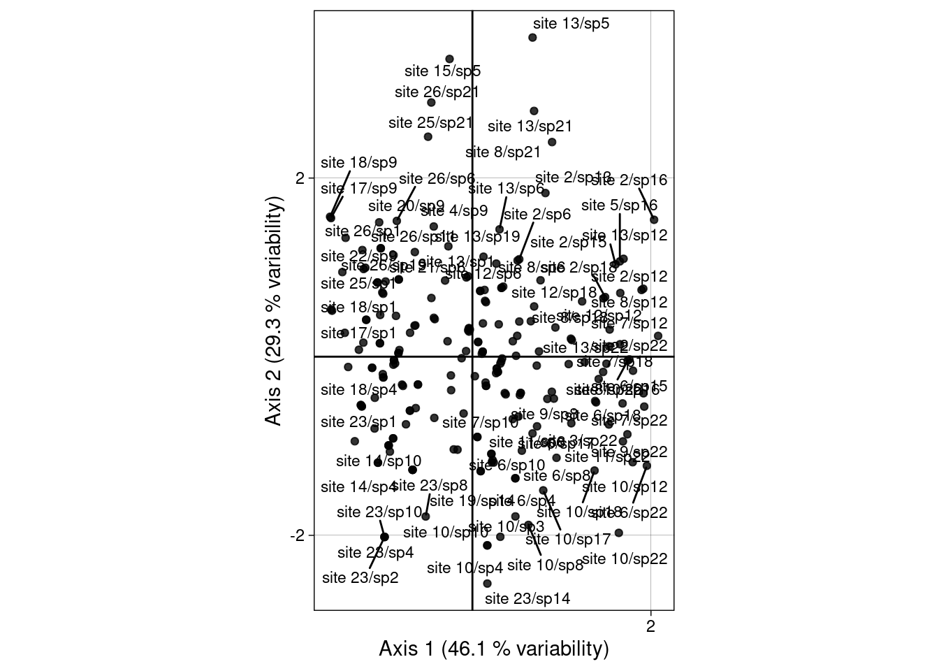
Once we have the correspondences scores, we can group them by row (site) or column (species) to compute conditional summary statistics:
These conditional statistics can be computed using \(H_k(i,j)\) (weighted means/variances/covariances) or using the dcCA scores. We only present the dcCA scores formulas below.
Formulas using dcCA scores
| Rows (sites) | Columns (species) | |
|---|---|---|
| Mean for axis \(k\) | \[m_k(i) = \frac{1}{\sqrt{2 \mu_k}} \times (LC1_k(i) + L_k(i))\] | \[m_k(j) = \frac{1}{\sqrt{2 \mu_k}} \times (CC1_k(j) + C_k(j))\] |
| Variance for axis \(k\) | \[s^2_k(i) = \frac{1}{2\lambda_k\mu_k} \left( \frac{1}{y_{i \cdot}} \sum_{j = 1}^c \left(y_{ij} CC_k^2(j) \right) - \lambda_k L_k^2(i) \right)\] | \[s^2_k(j) = \frac{1}{2\lambda_k\mu_k} \left( \frac{1}{y_{\cdot j}} \sum_{i = 1}^r \left(y_{ij} LC_k^2(i) \right) - \lambda_k C_k^2(j) \right)\] |
| Covariance between axes \(k\), \(l\) |
Let’s compare the means obtained from canonical correlations scores and the dcCA scores.
n <- sum(Y)Below is a graphical illustration of scoreRC grouped by rows:
s.class(scoreRC,
        wt = Yfreq0$Freq,
        fac = as.factor(Yfreq0$row),
        plabels.col = params$colsite,
        main = "With RC score (points = correspondences)")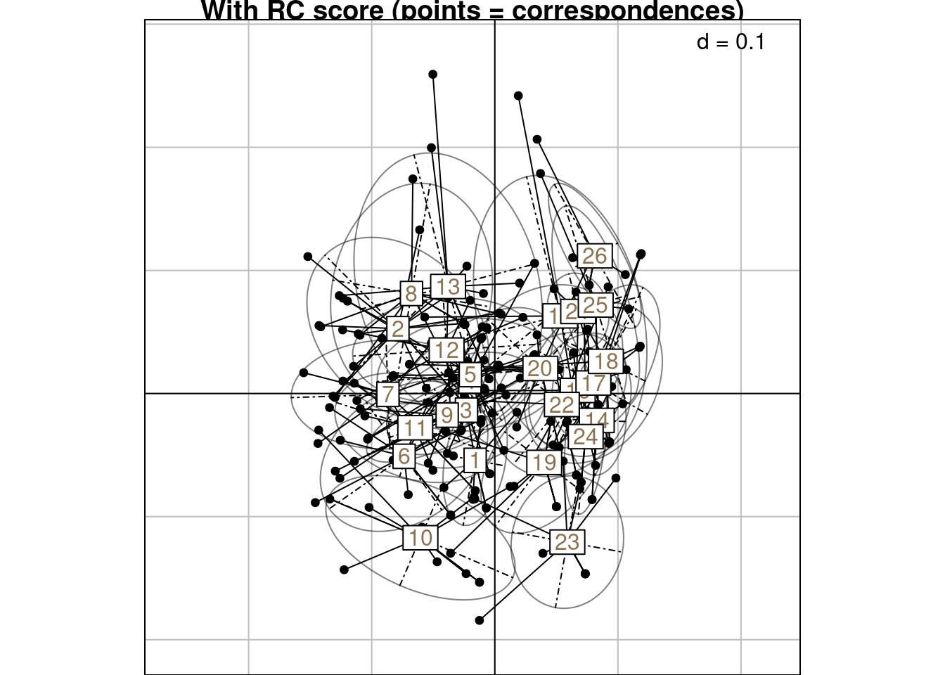
mrowsRC <- meanfacwt(scoreRC_scaled, fac = Yfreq0$row, wt = Yfreq0$Freq)
mrowsRC/(as.matrix(dcca$l1 + dcca$lsR) %*% diag(1/sqrt(2*mu_dcca)))
X1 X2 X3 X4 X5 X6
1 -1 1 -1 1 -1 -1
2 -1 1 -1 1 -1 -1
3 -1 1 -1 1 -1 -1
4 -1 1 -1 1 -1 -1
5 -1 1 -1 1 -1 -1
6 -1 1 -1 1 -1 -1
7 -1 1 -1 1 -1 -1
8 -1 1 -1 1 -1 -1
9 -1 1 -1 1 -1 -1
10 -1 1 -1 1 -1 -1
11 -1 1 -1 1 -1 -1
12 -1 1 -1 1 -1 -1
13 -1 1 -1 1 -1 -1
14 -1 1 -1 1 -1 -1
15 -1 1 -1 1 -1 -1
16 -1 1 -1 1 -1 -1
17 -1 1 -1 1 -1 -1
18 -1 1 -1 1 -1 -1
19 -1 1 -1 1 -1 -1
20 -1 1 -1 1 -1 -1
21 -1 1 -1 1 -1 -1
22 -1 1 -1 1 -1 -1
23 -1 1 -1 1 -1 -1
24 -1 1 -1 1 -1 -1
25 -1 1 -1 1 -1 -1
26 -1 1 -1 1 -1 -1varrowsRC <- varfacwt(scoreRC_scaled, fac = Yfreq0$row, wt = Yfreq0$Freq)# Get marginal counts
yi_ <- rowSums(Y)
y_j <- colSums(Y)
varrows_dcca <- matrix(nrow = r,
ncol = l)
for (i in 1:r) {
# Get CCA scores for site i
Li <- dcca$lsR[i, ]
# Compute the part with the sum on Cj
# we add all coordinates Cj^2 weighted by the number of observations on site i
sumCj <- t(Y[i, ]) %*% as.matrix(dcca$co)^2
# Fill i-th row with site i variance along each axis
varrows_dcca[i, ] <- (1/(2*lambda_dcca*mu_dcca)) * (((1/yi_[i])*sumCj) - lambda_dcca*as.numeric(Li)^2)
}varrowsRC/varrows_dcca X1 X2 X3 X4 X5 X6
1 1 1 1 1 1 1
2 1 1 1 1 1 1
3 1 1 1 1 1 1
4 1 1 1 1 1 1
5 1 1 1 1 1 1
6 1 1 1 1 1 1
7 1 1 1 1 1 1
8 1 1 1 1 1 1
9 1 1 1 1 1 1
10 1 1 1 1 1 1
11 1 1 1 1 1 1
12 1 1 1 1 1 1
13 1 1 1 1 1 1
14 1 1 1 1 1 1
15 1 1 1 1 1 1
16 1 1 1 1 1 1
17 1 1 1 1 1 1
18 1 1 1 1 1 1
19 1 1 1 1 1 1
20 1 1 1 1 1 1
21 1 1 1 1 1 1
22 1 1 1 1 1 1
23 1 1 1 1 1 1
24 1 1 1 1 1 1
25 1 1 1 1 1 1
26 1 1 1 1 1 1Below is an illustration of the RC scores grouped by species.
s.class(scoreRC,
        wt = Yfreq0$Freq,
        fac = as.factor(Yfreq0$colind),
        lab = colnames(Y),
        plabels.col = params$colspp,
        main = "With RC score (points = correspondences)")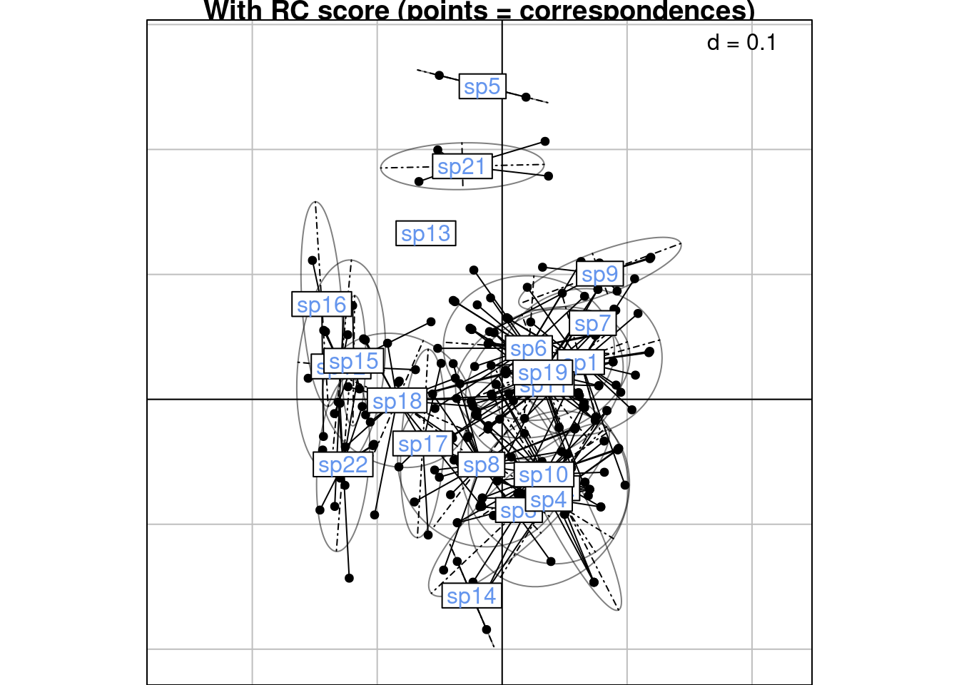
mcolsRC <- meanfacwt(scoreRC_scaled, fac = Yfreq0$colind, wt = Yfreq0$Freq)

mcolsRC/(as.matrix(dcca$lsQ + dcca$c1) %*% diag(1/sqrt(2*mu_dcca)))
X1 X2 X3 X4 X5 X6
1 -1 1 -1 1 -1 -1
2 -1 1 -1 1 -1 -1
3 -1 1 -1 1 -1 -1
4 -1 1 -1 1 -1 -1
5 -1 1 -1 1 -1 -1
6 -1 1 -1 1 -1 -1
7 -1 1 -1 1 -1 -1
8 -1 1 -1 1 -1 -1
9 -1 1 -1 1 -1 -1
10 -1 1 -1 1 -1 -1
11 -1 1 -1 1 -1 -1
12 -1 1 -1 1 -1 -1
13 -1 1 -1 1 -1 -1
14 -1 1 -1 1 -1 -1
15 -1 1 -1 1 -1 -1
16 -1 1 -1 1 -1 -1
17 -1 1 -1 1 -1 -1
18 -1 1 -1 1 -1 -1
19 -1 1 -1 1 -1 -1
20 -1 1 -1 1 -1 -1
21 -1 1 -1 1 -1 -1varcolsRC <- varfacwt(scoreRC_scaled, fac = Yfreq0$colind, wt = Yfreq0$Freq)varcols_dcca <- matrix(nrow = c,
ncol = l)
for (j in 1:c) {
# Get CCA scores for species j
Cj <- dcca$lsQ[j, ]
# Compute the part with the sum on Li
# we add all coordinates Li^2 weighted by the number of observations on species j
sumLi <- t(Y[, j]) %*% as.matrix(dcca$li)^2
# Fill i-th row with site i variance along each axis
varcols_dcca[j, ] <- (1/(2*lambda_dcca*mu_dcca)) * (((1/y_j[j])*sumLi) - lambda_dcca*as.numeric(Cj)^2)
}varcolsRC/varcols_dcca X1 X2 X3 X4 X5 X6
1 1 1 1 1 1 1
2 1 1 1 1 1 1
3 1 1 1 1 1 1
4 1 1 1 1 1 1
5 1 1 1 1 1 1
6 1 1 1 1 1 1
7 0 0 0 0 0 0
8 1 1 1 1 1 1
9 1 1 1 1 1 1
10 1 1 1 1 1 1
11 1 1 1 1 1 1
12 1 1 1 1 1 1
13 0 NaN 0 0 0 0
14 1 1 1 1 1 1
15 1 1 1 1 1 1
16 1 1 1 1 1 1
17 1 1 1 1 1 1
18 1 1 1 1 1 1
19 1 1 1 1 1 1
20 1 1 1 1 1 1
21 1 1 1 1 1 1For the scores computed with R scores and C scores, we have 3 types of formulas:
Here, we don’t show the definition.
Formulas using dcCA scores
| Rows (sites) | Columns (species) | |
|---|---|---|
| Mean for axis \(k\) | \[mR_k(i) = \frac{1}{\sqrt{n}} LC1_k(i)\] (\(LC1 =\) normed LC score ($l1)) |
\[mR_k(j) = \frac{1}{\sqrt{n}} C_k(j)\] (\(C =\) species WA score ($lsQ)) |
| Variance for axis \(k\) | None | \[sR_k^2(j) = \frac{1}{n\lambda_k} \left( \frac{1}{y_{\cdot j}} \sum_{i = 1}^r \left(y_{ij} LC_k^2(i) \right) - \lambda_k C_k^2(j) \right)\] |
| Covariance between axes \(k\), \(l\) |
| Rows (sites) | Columns (species) | |
|---|---|---|
| Mean for axis \(k\) | \[\frac{1}{\sqrt{n}} L_k(i)\] (\(L_k(i) =\) sites WA score ($lsR)) |
\[\frac{1}{\sqrt{n}} CC1_k(j)\] (\(CC1_k(j) =\) normed LC species score ($c1)) |
| Variance for axis \(k\) | \[sC_k^2(i) = \frac{1}{n\lambda_k} \left( \frac{1}{y_{i \cdot}} \sum_{j = 1}^c \left(y_{ij} CC_k^2(j) \right) - \lambda_k L_k^2(i) \right)\] | None |
| Covariance between axes \(k\), \(l\) |
Relation between RC scores and R score / C score
| Rows (sites) | Columns (species) | |
|---|---|---|
| Mean for axis \(k\) | \[mR_k(i) = \frac{\sqrt{2 \mu_k}}{\sqrt{n}} m_k(i) - \frac{1}{\sqrt{n}} L_k(i)\] | \[mR_k(j) = \frac{\sqrt{2 \mu_k}}{\sqrt{n}} m_k(j) - \frac{1}{\sqrt{n}} CC1_k(j)\] |
| Variance for axis \(k\) | None | \(sR^2_k(j) = \frac{2\mu_k}{n} s^2_k(j)\) |
| Covariance between axes \(k\), \(l\) |
| Rows (sites) | Columns (species) | |
|---|---|---|
| Mean for axis \(k\) | \[mC_k(i) = \frac{\sqrt{2 \mu_k}}{\sqrt{n}} m_k(i) - \frac{1}{\sqrt{n}} LC1_k(i)\] | \[mC_k(j) = \frac{\sqrt{2 \mu_k}}{\sqrt{n}} m_k(j) - \frac{1}{\sqrt{n}} C_k(j)\] |
| Variance for axis \(k\) | \(sC^2_k(i) = \frac{2\mu_k}{n} s^2_k(i)\) | None |
| Covariance between axes \(k\), \(l\) |
Below is a graphical illustration of scoreC grouped by rows:
s.class(scoreC,
        wt = Yfreq0$Freq,
        fac = as.factor(Yfreq0$row),
        ppoints.col = params$colspp,
        plabels.col = params$colsite,
        main = "With C score (points = species scores)")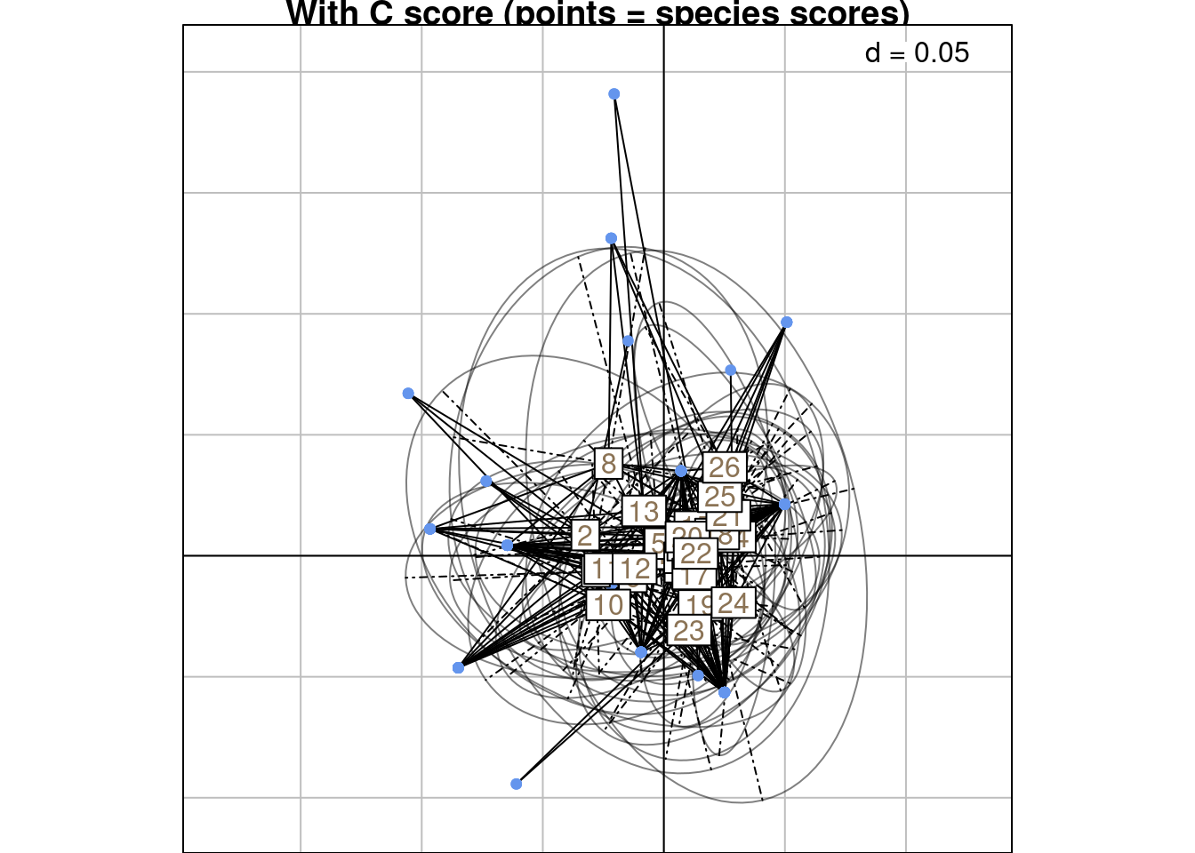
mrowsC <- meanfacwt(scoreC, fac = Yfreq0$row, wt = Yfreq0$Freq)

mrowsC/(dcca$lsR*1/sqrt(n))
Axis1 Axis2 Axis3 Axis4 Axis5 Axis6
1 -1 1 -1 1 -1 -1
2 -1 1 -1 1 -1 -1
3 -1 1 -1 1 -1 -1
4 -1 1 -1 1 -1 -1
5 -1 1 -1 1 -1 -1
6 -1 1 -1 1 -1 -1
7 -1 1 -1 1 -1 -1
8 -1 1 -1 1 -1 -1
9 -1 1 -1 1 -1 -1
10 -1 1 -1 1 -1 -1
11 -1 1 -1 1 -1 -1
12 -1 1 -1 1 -1 -1
13 -1 1 -1 1 -1 -1
14 -1 1 -1 1 -1 -1
15 -1 1 -1 1 -1 -1
16 -1 1 -1 1 -1 -1
17 -1 1 -1 1 -1 -1
18 -1 1 -1 1 -1 -1
19 -1 1 -1 1 -1 -1
20 -1 1 -1 1 -1 -1
21 -1 1 -1 1 -1 -1
22 -1 1 -1 1 -1 -1
23 -1 1 -1 1 -1 -1
24 -1 1 -1 1 -1 -1
25 -1 1 -1 1 -1 -1
26 -1 1 -1 1 -1 -1Now let’s compute the variance of scoreC per row:
varrowsC <- varfacwt(scoreC, fac = Yfreq0$row, wt = Yfreq0$Freq)Compare it to the variance of the RC score:
varrowsC[, 1:ncol(varrowsRC)]/(varrowsRC %*% diag(2*mu_dcca/n)) X1 X2 X3 X4 X5 X6
1 1 1 1 1 1 1
2 1 1 1 1 1 1
3 1 1 1 1 1 1
4 1 1 1 1 1 1
5 1 1 1 1 1 1
6 1 1 1 1 1 1
7 1 1 1 1 1 1
8 1 1 1 1 1 1
9 1 1 1 1 1 1
10 1 1 1 1 1 1
11 1 1 1 1 1 1
12 1 1 1 1 1 1
13 1 1 1 1 1 1
14 1 1 1 1 1 1
15 1 1 1 1 1 1
16 1 1 1 1 1 1
17 1 1 1 1 1 1
18 1 1 1 1 1 1
19 1 1 1 1 1 1
20 1 1 1 1 1 1
21 1 1 1 1 1 1
22 1 1 1 1 1 1
23 1 1 1 1 1 1
24 1 1 1 1 1 1
25 1 1 1 1 1 1
26 1 1 1 1 1 1Now, we compute the mean per row (site) from the row (sites) scores.
Below is a graphical illustration of scoreR grouped by rows:
s.class(scoreR,
        wt = Yfreq0$Freq,
        fac = as.factor(Yfreq0$row),
        ppoints.col = params$colsite,
        plabels.col = params$colsite,
        main = "With R score (points = sites scores)")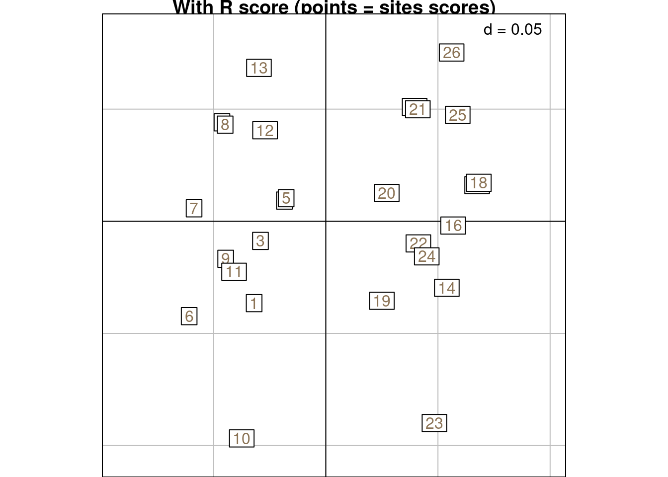
mrowsR <- meanfacwt(scoreR, fac = Yfreq0$row, wt = Yfreq0$Freq)

mrowsR/(dcca$l1*1/sqrt(n))
RS1 RS2 RS3 RS4 RS5 RS6
X1 -1 1 -1 1 -1 -1
X2 -1 1 -1 1 -1 -1
X3 -1 1 -1 1 -1 -1
X4 -1 1 -1 1 -1 -1
X5 -1 1 -1 1 -1 -1
X6 -1 1 -1 1 -1 -1
X7 -1 1 -1 1 -1 -1
X8 -1 1 -1 1 -1 -1
X9 -1 1 -1 1 -1 -1
X10 -1 1 -1 1 -1 -1
X11 -1 1 -1 1 -1 -1
X12 -1 1 -1 1 -1 -1
X13 -1 1 -1 1 -1 -1
X14 -1 1 -1 1 -1 -1
X15 -1 1 -1 1 -1 -1
X16 -1 1 -1 1 -1 -1
X17 -1 1 -1 1 -1 -1
X18 -1 1 -1 1 -1 -1
X19 -1 1 -1 1 -1 -1
X20 -1 1 -1 1 -1 -1
X21 -1 1 -1 1 -1 -1
X22 -1 1 -1 1 -1 -1
X23 -1 1 -1 1 -1 -1
X24 -1 1 -1 1 -1 -1
X25 -1 1 -1 1 -1 -1
X26 -1 1 -1 1 -1 -1The variance is null.
We group the scoreC per species. Below is an illustration:
s.class(scoreC,
        wt = Yfreq0$Freq,
        fac = as.factor(Yfreq0$colind),
        lab = colnames(Y),
        ppoints.col = params$colspp,
        plabels.col = params$colspp,
        main = "With C score (points = species scores)")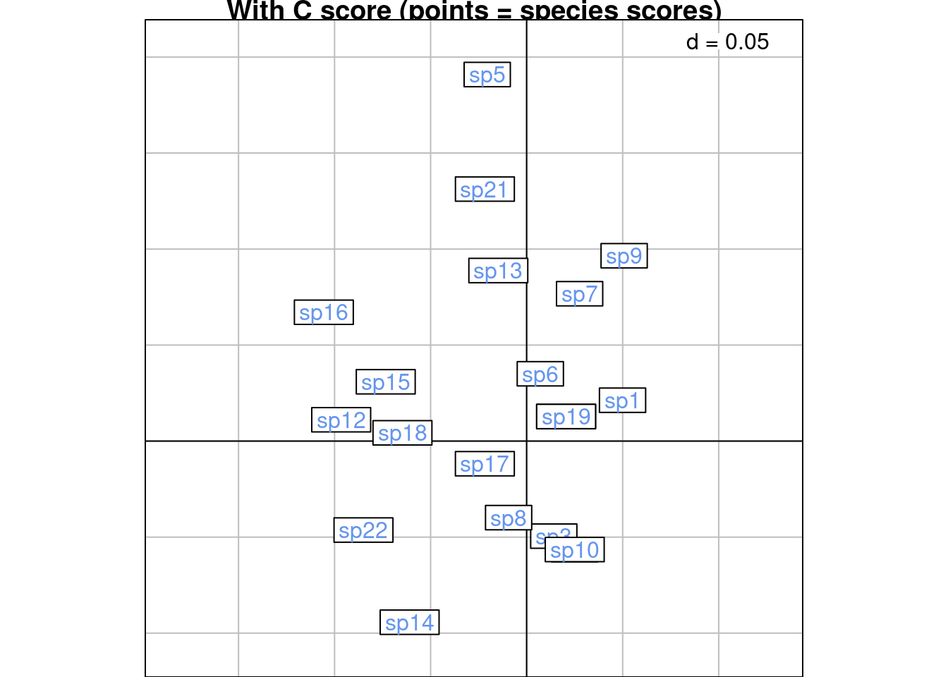
mcolsC <- meanfacwt(scoreC, fac = Yfreq0$colind, wt = Yfreq0$Freq)

mcolsC/(dcca$c1*1/sqrt(n))
CS1 CS2 CS3 CS4 CS5 CS6
sp1 -1 1 -1 1 -1 -1
sp2 -1 1 -1 1 -1 -1
sp3 -1 1 -1 1 -1 -1
sp4 -1 1 -1 1 -1 -1
sp5 -1 1 -1 1 -1 -1
sp6 -1 1 -1 1 -1 -1
sp7 -1 1 -1 1 -1 -1
sp8 -1 1 -1 1 -1 -1
sp9 -1 1 -1 1 -1 -1
sp10 -1 1 -1 1 -1 -1
sp11 -1 1 -1 1 -1 -1
sp12 -1 1 -1 1 -1 -1
sp13 -1 1 -1 1 -1 -1
sp14 -1 1 -1 1 -1 -1
sp15 -1 1 -1 1 -1 -1
sp16 -1 1 -1 1 -1 -1
sp17 -1 1 -1 1 -1 -1
sp18 -1 1 -1 1 -1 -1
sp19 -1 1 -1 1 -1 -1
sp21 -1 1 -1 1 -1 -1
sp22 -1 1 -1 1 -1 -1The variance is null.
Below are the scoreR grouped by column:
s.class(scoreR,
        wt = Yfreq0$Freq,
        fac = as.factor(Yfreq0$colind),
        lab = colnames(Y),
        ppoints.col = params$colsite,
        plabels.col = params$colspp,
        main = "With R score (points = sites scores)")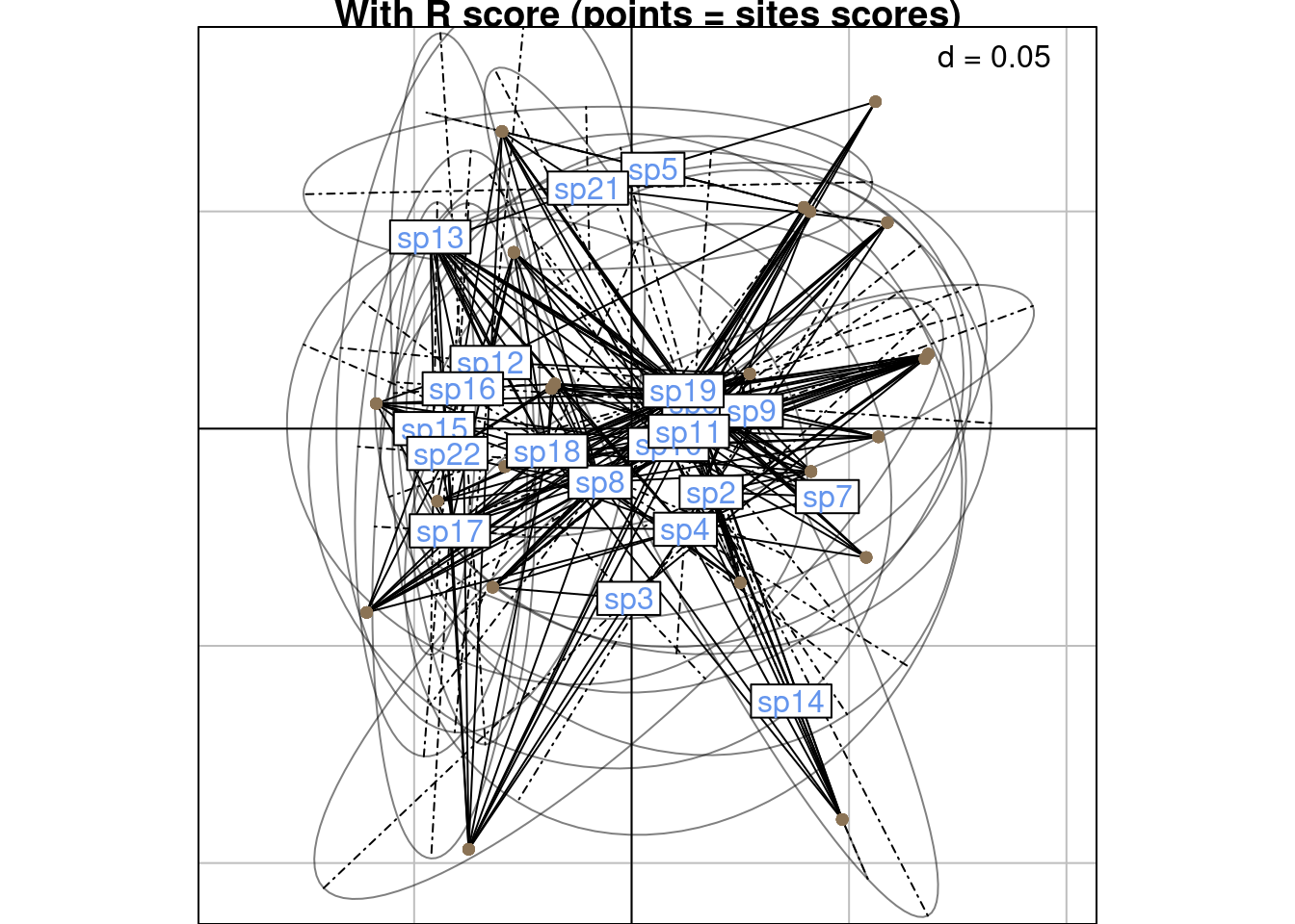
mcolsR <- meanfacwt(scoreR, fac = Yfreq0$colind, wt = Yfreq0$Freq)

mcolsR/(dcca$lsQ*1/sqrt(n))
Comp1 Comp2 Comp3 Comp4 Comp5 Comp6
sp1 -1 1 -1 1 -1 -1
sp2 -1 1 -1 1 -1 -1
sp3 -1 1 -1 1 -1 -1
sp4 -1 1 -1 1 -1 -1
sp5 -1 1 -1 1 -1 -1
sp6 -1 1 -1 1 -1 -1
sp7 -1 1 -1 1 -1 -1
sp8 -1 1 -1 1 -1 -1
sp9 -1 1 -1 1 -1 -1
sp10 -1 1 -1 1 -1 -1
sp11 -1 1 -1 1 -1 -1
sp12 -1 1 -1 1 -1 -1
sp13 -1 1 -1 1 -1 -1
sp14 -1 1 -1 1 -1 -1
sp15 -1 1 -1 1 -1 -1
sp16 -1 1 -1 1 -1 -1
sp17 -1 1 -1 1 -1 -1
sp18 -1 1 -1 1 -1 -1
sp19 -1 1 -1 1 -1 -1
sp21 -1 1 -1 1 -1 -1
sp22 -1 1 -1 1 -1 -1Now let’s compute the variance of scoreC per row:
varcolsR <- varfacwt(scoreR, fac = Yfreq0$colind, wt = Yfreq0$Freq)Compare it to the variance of the RC score:
varcolsR/(varcolsRC %*% diag(2*mu_dcca/n)) X1 X2 X3 X4 X5 X6
1 1 1 1 1 1 1
2 1 1 1 1 1 1
3 1 1 1 1 1 1
4 1 1 1 1 1 1
5 1 1 1 1 1 1
6 1 1 1 1 1 1
7 NaN NaN NaN NaN NaN NaN
8 1 1 1 1 1 1
9 1 1 1 1 1 1
10 1 1 1 1 1 1
11 1 1 1 1 1 1
12 1 1 1 1 1 1
13 NaN NaN NaN NaN NaN NaN
14 1 1 1 1 1 1
15 1 1 1 1 1 1
16 1 1 1 1 1 1
17 1 1 1 1 1 1
18 1 1 1 1 1 1
19 1 1 1 1 1 1
20 1 1 1 1 1 1
21 1 1 1 1 1 1The means of the RC scores by row (site) \(m_k(i)\) multiplied by a scaling factor \(\sqrt{2\mu_k}\) are equal to $lsR+$l1.
# Invert first column
mrowsRC_inv <- mrowsRC
mrowsRC_inv[, 1] <- -mrowsRC_inv[, 1]
(mrowsRC_inv[, 1:2] %*% diag(sqrt(2*mu_dcca[1:2])))/(dcca$l1[, 1:2]+dcca$lsR[, 1:2]) RS1 RS2
X1 1 1
X2 1 1
X3 1 1
X4 1 1
X5 1 1
X6 1 1
X7 1 1
X8 1 1
X9 1 1
X10 1 1
X11 1 1
X12 1 1
X13 1 1
X14 1 1
X15 1 1
X16 1 1
X17 1 1
X18 1 1
X19 1 1
X20 1 1
X21 1 1
X22 1 1
X23 1 1
X24 1 1
X25 1 1
X26 1 1However, perhaps it is more intuitive to see the \(m_k(i)\) as the mean between $lsR and $l1: for that, we divide \(m_k(i) \times \sqrt{2\mu_k}\) by 2.
The graph below shows \(\frac{m_k(i) \times \sqrt{2\mu_k}}{2}\) along with the sites LS and WA scores. They are superimposed to the mean between $lsR and $l1 on the graph below:
# Create a long df with $lsR and $l1 for the plot
bindlsR <- dcca$lsR
colnames(bindlsR) <- colnames(dcca$l1)
lscores <- rbind(dcca$l1, bindlsR)s.class(lscores,
fac = as.factor(rep(rownames(Y), 2)),
ppoints.col = params$colsite,
wt = rep(dcca$lw, 2),
plabels.col = params$colsite)
s.label((mrowsRC_inv %*% diag(sqrt(mu_dcca*2)/2)),
plabels.col = "darkorchid3",
add = TRUE)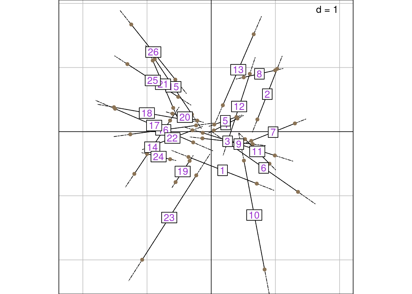
That was not too bad but it seems strange to compare LC1 and WA scores: LC and WA would be a better fit.
# Create a long df with $lsR and $l1 for the plot
bindlsR <- dcca$lsR
colnames(bindlsR) <- colnames(dcca$li)
lscores <- rbind(dcca$li, bindlsR)s.class(lscores,
fac = as.factor(rep(rownames(Y), 2)),
ppoints.col = params$colsite,
wt = rep(dcca$lw, 2),
plabels.col = params$colsite)
s.label((mrowsRC_inv %*% diag(sqrt(mu_dcca*lambda_dcca*2)/2)),
plabels.col = "darkorchid3",
add = TRUE)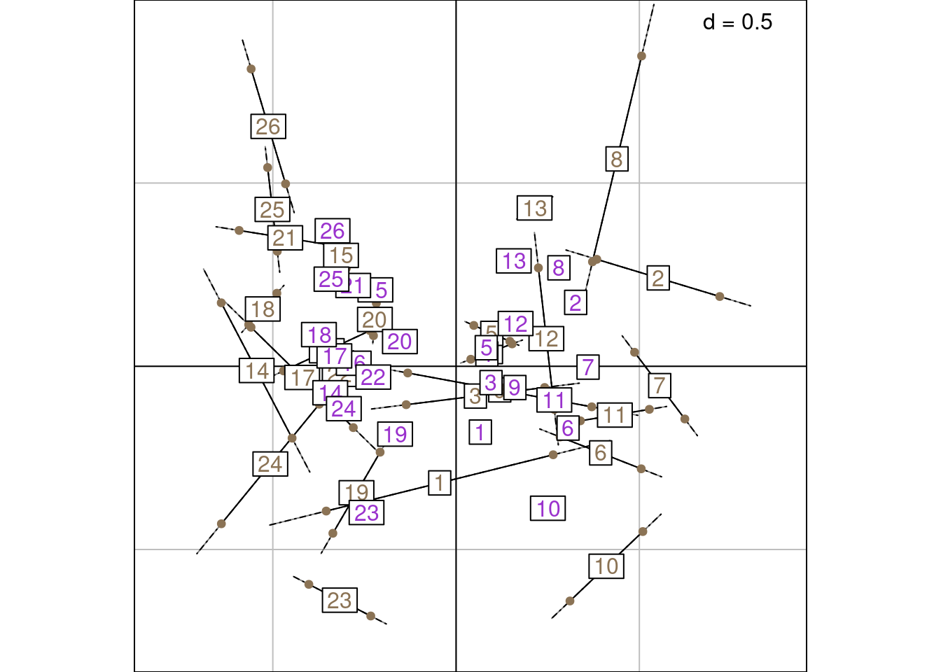
But then the mean of $lsR and $li is not superimposed to the means of the RC scores.
We can remain in the 2 biplots showing \(V\) with \(U^\star\) (c1 and lsR) (scaling type 1 = rows niches) and \(U\) and \(V^\star\) (lsQ and l1) (scaling type 2 = column niches).
To do that, we define the “CA-correspondences” \(h1_k(i, j)\) for scaling type 1:
\[h1_k(i, j) = \frac{u^\star_k(i) + v_k(j)}{2}\]
# Initialize results matrix
H1 <- matrix(nrow = nrow(Yfreq0),
             ncol = length(lambda_dcca))

for (k in 1:length(lambda_dcca)) { # For each axis
  ind <- 1 # initialize row index
  for (obs in 1:nrow(Yfreq0)) { # For each observation
    i <- Yfreq0$row[obs]
    j <- Yfreq0$col[obs]
    H1[ind, k] <- (dcca$lsR[i, k] + dcca$c1[j, k])/2
    ind <- ind + 1
  }
}corresp <- paste(Yfreq0$row, Yfreq0$col, sep = "-")
multiplot(indiv_row = as.data.frame(H1),
indiv_row_lab = corresp,
row_color = "black")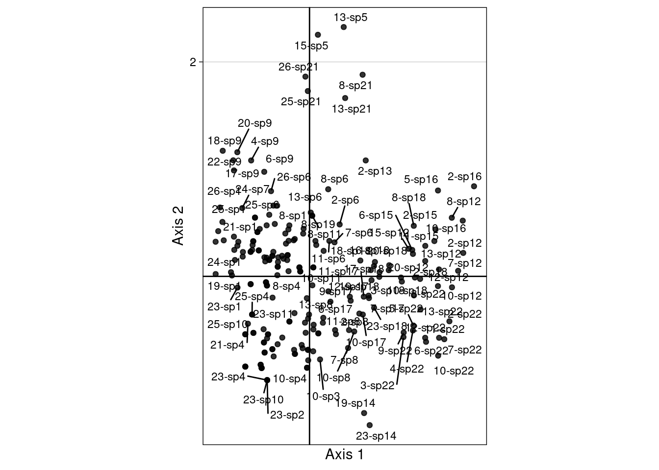
# Groupwise mean
mrows_nr <- meanfacwt(H1, fac = Yfreq0$row, wt = Yfreq0$Freq)
all(abs(abs(mrows_nr/dcca$lsR) - 1) < zero)
[1] TRUEhead(mrows_nr/mrowsRC) # It is different from the reciprocal scaling means X1 X2 X3 X4 X5 X6
1 1.6533866 0.5279337 0.5851892 -0.06781125 -0.1427069 -0.52991699
2 -0.6823573 0.2621430 -0.5942531 0.45270450 -0.5003293 -0.35482135
3 0.4415413 0.5643021 -0.5909733 -0.06788904 0.2459682 0.16148020
4 -0.1482127 0.1372513 -0.3383964 0.46228036 0.0820352 -0.32748383
5 -0.1818639 0.5279171 -0.2356614 0.11017165 -0.1671877 1.47696811
6 -0.2874715 0.2745043 -0.0337867 0.91463113 0.2885318 -0.05672653# Groupwise variance
varrows_nr <- varfacwt(H1, fac = Yfreq0$row, wt = Yfreq0$Freq)
res <- varrows_nr %*% diag(2/mu_dcca) # factor 2/mu
all(abs(res/varrowsRC - 1) < zero)[1] TRUE# We could also multiply H1 before computing the variance
H1_scaled <- H1 %*% diag(sqrt(2/mu_dcca)) # Factor sqrt(2/mu)
varrows_nr_scaled <- varfacwt(H1_scaled, fac = Yfreq0$row, wt = Yfreq0$Freq)
all(abs(varrows_nr_scaled/varrowsRC - 1) < zero)[1] TRUEs.class(H1,
fac = Yfreq0$row, plabels.col = params$colsite,
wt = Yfreq0$Freq,
main = "Non-reciprocal scaling")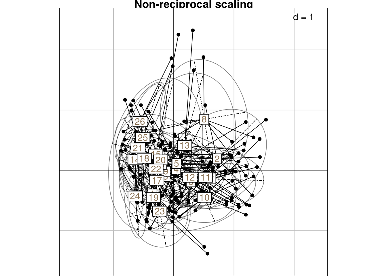
s.class(H,
        fac = Yfreq0$row, plabels.col = params$colsite,
        wt = Yfreq0$Freq,
        main = "Reciprocal scaling")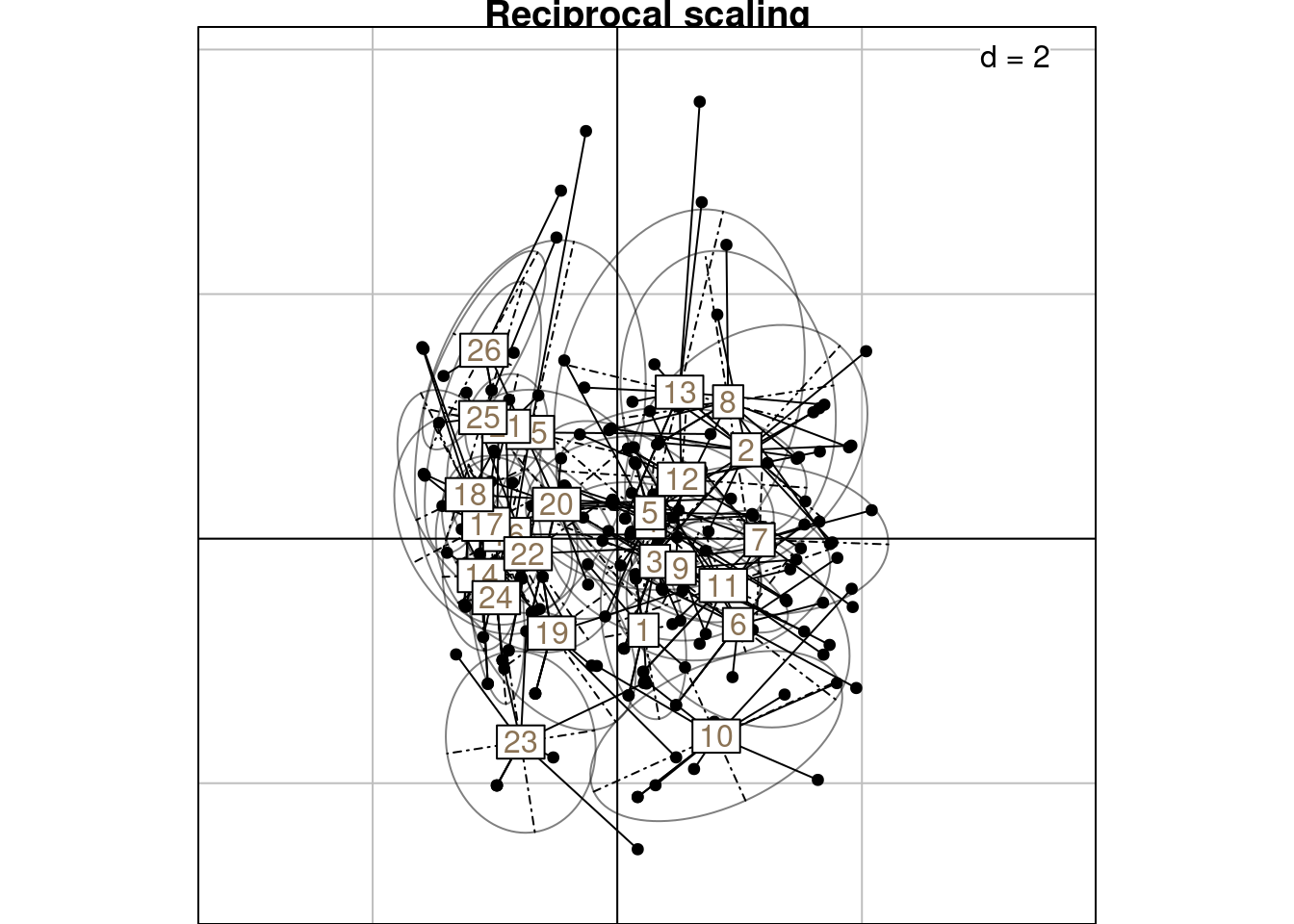
\(h1_k(i, j)\) can also be defined from the canonical correlation scores:
\[h1_k(i, j) = \frac{\sqrt{n} (R \bar{S_C} + S_C)}{2}\] where \(R \bar{S_C}\) corresponds to the duplicated version of \(\bar{S_C}\), the mean of C-scores by rows.
res <- meanfacwt(scoreC, fac = Yfreq0$row, wt = Yfreq0$Freq) # get the mean of scoreC by row
tabR <- as.matrix(acm.disjonctif(as.data.frame(Yfreq0$row)))
scoreRls <- tabR %*% res # Duplicate means according to correspondences of R

# Find back the formula from the scores
H1_cancor <- (sqrt(n)*(scoreRls[, 1:l] + scoreC[, 1:l]))/2
# H1_cancor_scaled <- scalewt(H1_cancor, wt = wt/sum(wt))

all(abs(abs(H1_cancor/H1) - 1) < zero)
[1] TRUEWe define the “CA-correspondences” \(h2_k(i, j)\) for scaling type 2:
\[h2_k(i, j) = \frac{u_k(i) + v^\star_k(j)}{2}\]
# Initialize results matrix
H2 <- matrix(nrow = nrow(Yfreq0),
             ncol = length(lambda_dcca))

for (k in 1:length(lambda_dcca)) { # For each axis
  ind <- 1 # initialize row index
  for (obs in 1:nrow(Yfreq0)) { # For each observation
    i <- Yfreq0$row[obs]
    j <- Yfreq0$col[obs]
    H2[ind, k] <- (dcca$l1[i, k] + dcca$lsQ[j, k])/2
    ind <- ind + 1
  }
}corresp <- paste(Yfreq0$row, Yfreq0$col, sep = "-")
multiplot(indiv_row = as.data.frame(H2),
indiv_row_lab = corresp,
row_color = "black")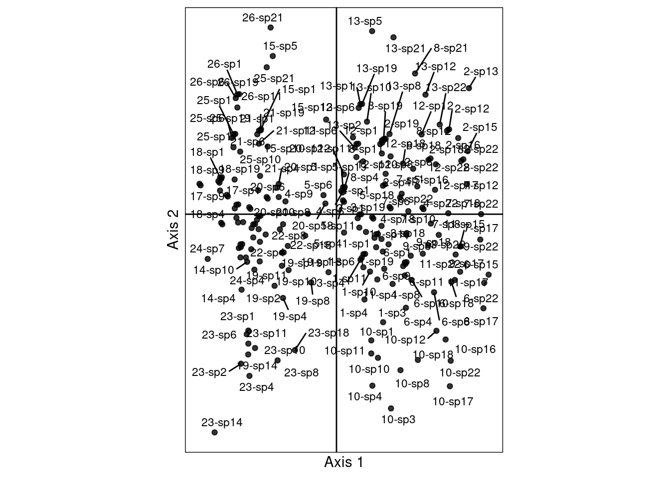
# Groupwise mean
mcols_nr <- meanfacwt(H2, fac = Yfreq0$col, wt = Yfreq0$Freq)
all(abs(abs(mcols_nr/dcca$lsQ)-1) < zero)
[1] TRUEhead(mcols_nr/mcolsRC) # It is different from the reciprocal scaling means X1 X2 X3 X4 X5 X6
sp1 -0.34539825 0.4613888 -0.1291876 0.59460911 0.05862701 -0.06963278
sp2 -0.69971219 0.3321361 -0.7654332 18.27788124 -0.85018616 -1.39038985
sp3 0.08000112 0.7109524 -0.3302009 0.40289677 -1.17113661 -0.25880816
sp4 -0.54804851 0.4688067 -0.2190234 0.75729851 0.70129907 -1.27143300
sp5 0.52038835 0.3837661 -0.3593968 -0.03308342 -0.76039465 -2.17864998
sp6 -1.10639827 0.2343722 -5.0626170 -0.15807737 -0.18222986 0.02268947# Groupwise variance
sp1 <- c(7, 13) # Species only present in one site
varcols_nr <- varfacwt(H2, fac = Yfreq0$col, wt = Yfreq0$Freq)
res <- varcols_nr %*% diag(2/mu_dcca)
all(abs(res[-sp1, ]/varcolsRC[-sp1, ] - 1) < zero) # Factor 2/mu[1] TRUEfac_col <- Yfreq0$col
s.class(H2,
fac = fac_col, plabels.col = params$colspp,
wt = Yfreq0$Freq,
main = "Non-reciprocal scaling")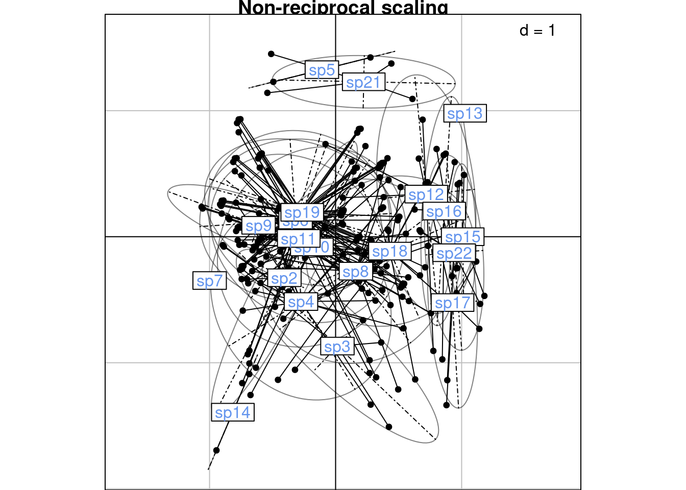
s.class(H,
        fac = fac_col, plabels.col = params$colspp,
        wt = Yfreq0$Freq,
        main = "Reciprocal scaling")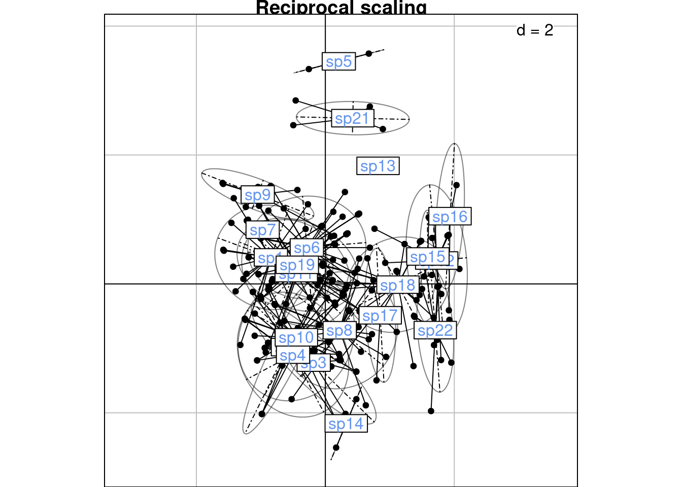
\(h2_k(i, j)\) can also be defined from the canonical correlation scores:
\[h2_k(i, j) = \frac{\sqrt{n} (S_R + C \bar{S_R})}{2}\]
where \(C \bar{S_R}\) corresponds to the duplicated version of \(\bar{S_R}\), the mean of R-scores by columns.
# ScoreR = l1
# ScoreC = c1
# mean of score C = ls

res <- meanfacwt(scoreR, fac = Yfreq0$col, wt = Yfreq0$Freq) # get the mean of scoreR by col
tabC <- as.matrix(acm.disjonctif(as.data.frame(Yfreq0$col)))
scoreCls <- tabC %*% res # Duplicate means according to correspondences of R

# Find back the formula from the scores
H2_cancor <- (sqrt(n)*(scoreR[, 1:l] + scoreCls[, 1:l]))/2

all(abs(abs(H2_cancor/H2) - 1) < zero)
[1] TRUE