Code
# Paths
library(here)

# Multivariate analysis
library(ade4)
library(adegraphics)

# Matrix algebra
library(expm)

# Plots
library(CAnetwork)
library(patchwork)
library(ggplot2)# Paths
library(here)
# Multivariate analysis
library(ade4)
library(adegraphics)
# Matrix algebra
library(expm)
# Plots
library(CAnetwork)
library(patchwork)
library(ggplot2)# Define bound for comparison to zero
zero <- 10e-10#' Normalize row or columns vectors of a matrix
#'
#' @param M the matrix to normalize
#' @param margin the margin (1 = rows, 2 = columns)
#'
#' @return The normalized matrix M
normalize <- function(M, margin) {
m_norm <- apply(M,
margin,
function(x) sqrt(sum(x^2)))
M_norm <- sweep(M, margin, m_norm, "/")
return(M_norm)
}The contents of this page relies heavily on Braak, Šmilauer, and Dray (2018).
Double constrained correspondence analysis (dc-CA) was developed as a natural extension of CCA and has been used to study the relationship between species traits and environmental variables.
In dc-CA, we have 3 matrices:
dat <- readRDS(here("data/Barbaro2012.rds"))
Y <- dat$comm
E <- dat$envir
T_ <- dat$traits

r <- dim(Y)[1]
c <- dim(Y)[2]
l <- dim(E)[2]
k <- dim(T_)[2]

plotmat(r = r, c = c,
        E = TRUE, T_ = TRUE,
        l = l, k = k)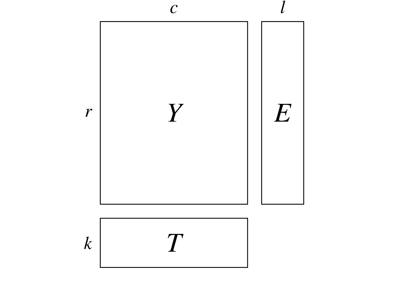
The aim of dc-CA is to find a linear combination of the predictor variables in \(E\) and \(T\) (environmental variables and traits) that maximizes the correlation.
Below are the first lines of these matrices for our data:
\(Y =\)
knitr::kable(head(Y))| sp1 | sp2 | sp3 | sp4 | sp5 | sp6 | sp7 | sp8 | sp9 | sp10 | sp11 | sp12 | sp13 | sp14 | sp15 | sp16 | sp17 | sp18 | sp19 | sp21 | sp22 |
|---|---|---|---|---|---|---|---|---|---|---|---|---|---|---|---|---|---|---|---|---|
| 1 | 0 | 1 | 1 | 0 | 1 | 0 | 2 | 0 | 1 | 1 | 0 | 0 | 0 | 0 | 0 | 0 | 0 | 1 | 0 | 0 |
| 2 | 0 | 0 | 2 | 0 | 1 | 0 | 5 | 0 | 2 | 0 | 2 | 4 | 0 | 3 | 3 | 0 | 3 | 1 | 0 | 2 |
| 5 | 0 | 0 | 2 | 0 | 1 | 0 | 2 | 0 | 1 | 2 | 0 | 0 | 0 | 0 | 0 | 0 | 3 | 2 | 0 | 1 |
| 3 | 0 | 0 | 0 | 0 | 1 | 0 | 4 | 1 | 0 | 1 | 0 | 0 | 0 | 0 | 0 | 0 | 2 | 0 | 0 | 1 |
| 5 | 0 | 0 | 1 | 0 | 1 | 0 | 2 | 0 | 0 | 3 | 0 | 0 | 0 | 0 | 1 | 0 | 3 | 1 | 0 | 1 |
| 1 | 0 | 0 | 1 | 0 | 2 | 0 | 3 | 1 | 2 | 1 | 0 | 0 | 0 | 1 | 0 | 1 | 2 | 2 | 0 | 3 |
\(E =\)
knitr::kable(head(E))| location | elevation | patch_area | perc_forests | perc_grasslands | ShannonLandscapeDiv |
|---|---|---|---|---|---|
| 0 | 10 | 6.28 | 7.7882 | 67.7785 | 0.232 |
| 0 | 30 | 7.92 | 16.4129 | 43.4066 | 0.274 |
| 0 | 430 | 83.24 | 24.4526 | 28.4995 | 0.274 |
| 0 | 420 | 140.83 | 41.9966 | 34.2412 | 0.260 |
| 0 | 400 | 140.83 | 41.9966 | 34.2412 | 0.260 |
| 0 | 500 | 0.50 | 7.5445 | 67.0780 | 0.240 |
\(T =\)
knitr::kable(head(T_))| biog | forag | mass | diet | move | nest | eggs | |
|---|---|---|---|---|---|---|---|
| sp1 | 1 | 2 | 2 | 3 | 1 | 2 | 2 |
| sp2 | 1 | 1 | 1 | 2 | 1 | 2 | 2 |
| sp3 | 1 | 1 | 2 | 2 | 2 | 2 | 1 |
| sp4 | 1 | 1 | 1 | 2 | 1 | 2 | 2 |
| sp5 | 1 | 3 | 3 | 1 | 2 | 3 | 4 |
| sp6 | 1 | 1 | 4 | 3 | 2 | 2 | 1 |
(r <- dim(Y)[1])[1] 26(c <- dim(Y)[2])[1] 21(l <- dim(E)[2])[1] 6(k <- dim(T_)[2])[1] 7dc-CA must not have to many traits compared to species: that is a disadvantage compared to RLQ, but on the other hand dc-CA allows to see relationships that RLQ would miss (Braak, Šmilauer, and Dray 2018).
There are several ways to perform dc-CA (Braak, Šmilauer, and Dray 2018), notably:
We define matrix \(D\) as:
\[D = [\tilde{E}^\top D_r \tilde{E}]^{-1/2} \tilde{E}^\top P_0 \tilde{T} [\tilde{T}^\top D_c \tilde{T}]^{-1/2}\]
Note: contrary to Braak, Šmilauer, and Dray (2018), in this document we use the matrix \(P_0\) instead of \(Y\).
We perform the SVD of \(D\):
\[ D = B_0 \Delta C_0^\top \]
This allows us to find the eigenvectors \(B_0\) (regression coefficients multiplying rows/environment variables) and \(C_0\) (regression coefficients multiplying columns/species traits).
The eigenvalues of the dc-CA are the squared eigenvalues of the SVD: \(\Lambda = \Delta^2\).
There are \(\min(k, l)\) non-null eigenvalues???
Transformation of \(B_0\) and \(C_0\)
Then, we transform \(B_0\) and \(C_0\) (scaling):
Individuals coordinates
The individuals coordinates (species or sites) can be computed in two ways:
Linear combinations (LC scores) are computed from those coefficients :
Weighted averages (WA scores) are computed from the scores of the other individuals:
To check our results, we first perform a dc-CA with ade4:
ca <- dudi.coa(Y,
               nf = c-1,
               scannf = FALSE)

dcca <- dpcaiv2(dudi = ca,
                dfR = E,
                dfQ = T_,
                scannf = FALSE,
nf = min(k, l))We define \(P\) as the relative counts of \(Y\) and \(P_0\) as its centered scaled version:
P <- Y/sum(Y)

# Initialize P0 matrix
P0 <- matrix(ncol = ncol(Y), nrow = nrow(Y))
colnames(P0) <- colnames(Y)
rownames(P0) <- rownames(Y)

for(i in 1:nrow(Y)) { # For each row
  for (j in 1:ncol(Y)) { # For each column
    # Do the sum
    pi_ <- sum(P[i, ])
    p_j <- sum(P[, j])

    # Compute the transformation
    P0[i, j] <- (P[i, j] - (pi_*p_j))/sqrt(pi_*p_j)
  }
}
First, we need to center-scale the traits and environment matrices (resp. \(\tilde{T}\) and \(\tilde{E}\)). To do so, we use the occurrences in matrix \(P\) as weights:
E_wt <- rowSums(P)/nrow(E)
Escaled <- scalewt(E, wt = E_wt, scale = TRUE)

T_wt <- colSums(P)/nrow(T_)
Tscaled <- scalewt(T_, wt = T_wt, scale = TRUE)
# Check centering
M1 <- matrix(rep(1, nrow(P)), nrow = 1)
all(abs(M1 %*% diag(rowSums(P)) %*% Escaled) < zero)[1] TRUEM1 <- matrix(rep(1, ncol(P)), nrow = 1)
all(abs(M1 %*% diag(colSums(P)) %*% Tscaled) < zero)[1] TRUEThis is equivalent to scaling “inflated” versions of these matrices matching the occurrence counts in \(P\) (below).
\[ \tilde{E} = \frac{E - \bar{E}_{infl}}{\sigma_{Einfl}} \]
\[ \tilde{T} = \frac{T - \bar{T}_{infl}}{\sigma_{Tinfl}} \]
# Center E -----
pi_ <- rowSums(P)
Escaled2 <- matrix(nrow = nrow(E), ncol = ncol(E))

for(i in 1:ncol(Escaled)) {
  emean <- sum(E[, i]*pi_/sum(P))
  Escaled2[, i] <- (E[, i] - emean)/(sqrt(sum(pi_*(E[, i] - emean)^2)))
}
# This is the same as computing a mean on inflated data matrix Einfl and centering E with these means

# Center T -----
p_j <- colSums(P)
Tscaled2 <- matrix(nrow = nrow(T_), ncol = ncol(T_))
rownames(Tscaled2) <- rownames(T_)
colnames(Tscaled2) <- colnames(T_)

for(j in 1:ncol(Tscaled)) {
  tmean <- sum(T_[, j]*p_j/sum(P))
  Tscaled2[, j] <- (T_[, j] - tmean)/(sqrt(sum(p_j*(T_[, j] - tmean)^2)))
}# Check equivalence between the 2 methods
all(abs(Escaled/Escaled2 - 1) < zero)[1] TRUEall(abs(Tscaled/Tscaled2 - 1) < zero)[1] TRUEThen, we search scores \(u\) and \(v\) that maximize the fourth-corner correlation \(u^\top P v\) (where \(u\) are the sites (rows) scores and \(v\) are the species (columns) scores).
In this framework, we define \(u\) and \(v\) as linear combinations of traits and environmental variables: \(u = \tilde{E}b\) and \(v = \tilde{T}c\).
So in the end, we need to maximize \(u^\top P_0 v\) with respect to the coefficients vectors \(b\) and \(c\):
\[ \max_{b, c}(u^\top P v) = \max_{b, c}\left(\left[\tilde{E}b\right]^\top P \tilde{T}c \right) \]
These equations are written for the first axis, but we can also write them in matrix form:
\[ \max_{B, C}(U^\top P V) = \max_{B, C}\left(\left[\tilde{E}B\right]^\top P \tilde{T}C \right) \]
We define the diagonal matrices \(D_r\) and \(D_c\), which contain the column and row sums of \(P\) (respectively). We introduce the following constraint on \(U\) and \(V\): \(u^\top D_r u = 1\) and \(v^\top D_c v = 1\). It means that the matrices \(U\) and \(V\) are orthonormal with respect to the weights \(D_r\) and \(D_c\). (In fact, these constraints will be relaxed later depending on the scaling (see below)).
To find the coefficients \(B\) and \(C\) defined above, we can perform a SVD or two diagonalizations (see below).
To find the coefficients \(B\) and \(C\), we perform the SVD of a matrix \(D\) defined as:
\[ D = \underbrace{[\tilde{E}^\top D_r \tilde{E}]^{-1/2}}_{L^{-1/2}} \underbrace{\tilde{E}^\top P \tilde{T}}_{R} \underbrace{[\tilde{T}^\top D_c \tilde{T}]^{-1/2}}_{K^{-1/2}} \]
# Define weights
dr <- rowSums(P)
dc <- colSums(P)

Dr <- diag(dr)
Dc <- diag(dc)
# Define intermediate matrices
L <- t(Escaled) %*% Dr %*% Escaled
R <- t(Escaled) %*% P %*% Tscaled
K <- t(Tscaled) %*% Dc %*% TscaledWith our dataset:
D <- solve(sqrtm(t(Escaled) %*% Dr %*% Escaled)) %*%
  t(Escaled) %*% P %*% Tscaled %*%
  solve(sqrtm(t(Tscaled) %*% Dc %*% Tscaled))
We perform the SVD of \(D\):
\[D = B_0 \Delta C_0^\top\]
sv <- svd(D)

# Singular values
delta <- sv$d
Delta <- diag(delta)

# Eigenvalues
lambda <- delta^2
Lambda <- diag(lambda)

# Eigenvectors
B0 <- sv$u
dim(B0) # l x l
[1] 6 6C0 <- sv$v
dim(C0) # k x l[1] 7 6Equivalently, we can also diagonalize the matrices \(M\) and \(M_2\) defined below.
\(M\) is defined as:
\[ M = [\underbrace{\tilde{E}^\top D_r \tilde{E}}_{L} ]^{-1} \underbrace{\tilde{E}^\top P \tilde{T}}_{R} [ \underbrace{\tilde{T}^\top D_c \tilde{T}}_{K} ]^{-1} \underbrace{\tilde{T}^\top P^\top \tilde{E}}_{R^\top} \tag{1}\]
We can also view \(M\) as:
\[ M = \underbrace{\left[\tilde{E}^\top D_r \tilde{E} \right]^{-1} \tilde{E}^\top P \tilde{T}}_{\hat{E}_{center} = \beta \tilde{T}} \underbrace{\left[\tilde{T}^\top D_c \tilde{T} \right]^{-1} \tilde{T}^\top P^\top \tilde{E}}_{\hat{T}_{center} = \gamma \tilde{E}} \]
where \(\hat{E}_{center}\) is the predicted values of sites variables from species traits. Reciprocally, \(\hat{T}_{center}\) is the predicted values of species traits from sites variables. \(\beta\) and \(\gamma\) are the vectors of the regression coefficients. From Equation 1, we have \(\beta = \left[\tilde{E}^\top D_r \tilde{E} \right]^{-1} \tilde{E}^\top P\) and \(\gamma = \left[\tilde{T}^\top D_c \tilde{T} \right]^{-1} \tilde{T}^\top P^\top\).
M <- solve(t(Escaled) %*% Dr %*% Escaled) %*% t(Escaled) %*% P %*% Tscaled %*% solve(t(Tscaled) %*% Dc %*% Tscaled) %*% t(Tscaled) %*% t(P) %*% Escaled\(M_2\) is defined as:
\[ M_2 = \underbrace{\left[\tilde{T}^\top D_c \tilde{T} \right]^{-1} \tilde{T}^\top P^\top \tilde{E}}_{\hat{T}_{center} = \gamma \tilde{E}} \underbrace{\left[\tilde{E}^\top D_r \tilde{E} \right]^{-1} \tilde{E}^\top P \tilde{T}}_{\hat{E}_{center} = \beta \tilde{T}} \]
M2 <- solve(t(Tscaled) %*% Dc %*% Tscaled) %*% t(Tscaled) %*% t(P) %*% Escaled %*% solve(t(Escaled) %*% Dr %*% Escaled) %*% t(Escaled) %*% P %*% Tscaled The eigenvectors matrices of these diagonalizations give us \(B\) and \(C\):
\[ M = B \Lambda_b B^{-1} \]
# Diagonalize M
eigB <- eigen(M)
lambdaB <- eigB$values
lambdaB # All l = 6 non-null eigenvectors
[1] 0.139487442 0.088736680 0.049183623 0.013797529 0.008736645 0.002485683B_diag <- eigB$vectors
# Check that the result checks out with SVD
all(abs(abs(B_diag/B0) - 1) < zero) # it isn't equal[1] FALSEapply(B_diag, 2, function(x) sqrt(sum(x^2))) # but B_diag is of norm 1 (like B0)[1] 1 1 1 1 1 1\[ M_2 = C \Lambda_c C^{-1} \]
# Diagonalize M2
eigC <- eigen(M2)
lambdaC <- eigC$values
lambdaC # l = 6 non-null eigenvalues
[1] 1.394874e-01 8.873668e-02 4.918362e-02 1.379753e-02 8.736645e-03
[6] 2.485683e-03 -1.180064e-17C_diag <- eigC$vectors
# Check that the result checks out with SVD
all(abs(abs(C_diag[, 1:l]/C0) - 1) < zero) # it isn't equal[1] FALSEapply(C_diag[, 1:l], 2, function(x) sqrt(sum(x^2))) # but C_diag is of norm 1 (like C0)[1] 1 1 1 1 1 1# The two diagonalizations have the same non-null eigenvectors
all(lambdaB - lambdaC[1:l] < zero)[1] TRUEThe eigenvalues of the SVD \(\Lambda = \Delta^2\) are the same as \(\Lambda_b\) and \(\Lambda_c\).
all(abs(lambda - lambdaB) < zero)[1] TRUEWe also define the following “scalings” for the coefficients:
\[ \left\{ \begin{array}{ll} B &= L^{-1/2} B_0\\ C &= K^{-1/2} C_0 \end{array} \right. \]
(We recall that \(L = \tilde{E}^\top D_r \tilde{E}\) and \(K = \tilde{T}^\top D_c \tilde{T}\)).
B <- solve(sqrtm(L)) %*% B0
C <- solve(sqrtm(K)) %*% C0
# B0 and C0 are of norm 1
apply(B0, 2, function(x) sqrt(sum(x^2))) [1] 1 1 1 1 1 1apply(C0, 2, function(x) sqrt(sum(x^2))) [1] 1 1 1 1 1 1# B and C are normed with L and K
# t(B) L B is the identity matrix
id_l <- diag(1, nrow = l, ncol = l)
all(abs((t(B) %*% L %*% B) - id_l) < zero)[1] TRUE# t(C) K C is the identity matrix
id_c <- diag(c(rep(1, k-1), 0),
nrow = k, ncol = k) # Identity minus last vector (zero)
C_k <- cbind(C, rep(0, k)) # Add null eigenvector
all(abs(t(C_k) %*% K %*% C_k - id_c) < zero)[1] TRUEUsing the coefficients \(B\) and \(C\), we can now define scores for sites and species scores as a linear combination of their variables:
U <- Escaled %*% B0

# Check it is the same as ade4 scores
all(abs(U/dcca$l1) - 1 < zero)
[1] FALSEV <- Tscaled %*% C
# Check it is the same as ade4 scores
all(abs(V/dcca$c1) - 1 < zero)[1] TRUEWe can also define species scores as the mean of sites LC scores (and the reverse):
Ustar <- solve(Dr) %*% P %*% V

# Check it is the same as ade4 scores
all(abs(Ustar/dcca$lsR) - 1 < zero)
[1] TRUEVstar <- solve(Dc) %*% t(P) %*% U
# Check it is the same as ade4 scores
all(abs(Vstar/dcca$lsQ) - 1 < zero)[1] FALSEThere are two types of coordinates: linear combination scores (LC scores) and weighted averages scores (WA scores) for the sites and species individuals.
The general formulas are:
In these formulas, note that the WA scores for one dimension are computed from the predicted scores of the other dimension.
Scaling type 1 (\(\alpha = 1\))
li)c1)lsR)Scaling type 2 (\(\alpha = 0\))
l1)co)lsQ)Scaling type 3 (\(\alpha = 1/2\))
\(\alpha\) changes the interpretation of the correlations vectors:
When plotting the correlation circle, to look at the correlations between variables of the same set (traits or environmental variables), we should use \(BS_{B2}\) and \(BS_{C1}\). There are the scores returned by ade4.
This type of scaling preserves the distances between rows (\(\alpha = 1\)).
With the scaling type 1, \(BS_{B1}\) represents the correlation between environmental variables and species and \(BS_{C1}\) represents the correlation between species traits and species.
# LC scores
U1 <- Escaled %*% B %*% Delta # rows
V1 <- Tscaled %*% C # columns

# WA scores
Ustar1 <- solve(Dr) %*% P %*% V # rows
Vstar1 <- solve(Dc) %*% t(P) %*% U  # columns

# # Variables scores
BS_B1 <- B %*% Delta
BS_C1 <- C

# Normalize
BS_B1norm <- normalize(BS_B1, 1)
BS_C1norm <- normalize(BS_C1, 1)

BS_C1 <- t(Tscaled) %*% Dc %*% V
# Compare results to ade4
all(abs(U1/dcca$li) - 1 < zero) # sites LC[1] TRUEall(abs(V1/dcca$c1) - 1 < zero) # spp LC[1] TRUEall(abs(Ustar1/dcca$lsR) - 1 < zero) # sites WA[1] TRUEall(abs(abs(Vstar1/dcca$lsQ) - 1) < zero) # not stored in ade4[1] FALSEall(abs(abs(BS_C1/dcca$corQ) - 1) < zero)[1] TRUEWe can either plot:
li) and species as \(V_1\) (c1) (left)lsR) and species as \(V_1\) (c1) (right)# LC scores
glc <- multiplot(indiv_row = U1, # LC for sites
indiv_col = V1, # LC1 for spp
indiv_row_lab = rownames(Y), indiv_col_lab = colnames(Y),
# var_row = BS_B1norm, var_row_lab = colnames(E),
# var_col = BS_C1norm, var_col_lab = colnames(T_),
row_color = params$colsite, col_color = params$colspp,
eig = lambda) +
ggtitle("Sites LC scores with species\nnormed at 1")
# WA scores
gwa <- multiplot(indiv_row = Ustar1, # WA for sites
indiv_col = V1, # LC1 for spp
indiv_row_lab = rownames(Y), indiv_col_lab = colnames(Y),
# var_row = BS_B1norm, var_row_lab = colnames(E),
# var_col = BS_C1norm, var_col_lab = colnames(T_),
row_color = params$colsite, col_color = params$colspp,
eig = lambda) +
ggtitle("Sites WA scores with species\nnormed at 1")
glc + gwa +
plot_layout(axis_titles = "collect")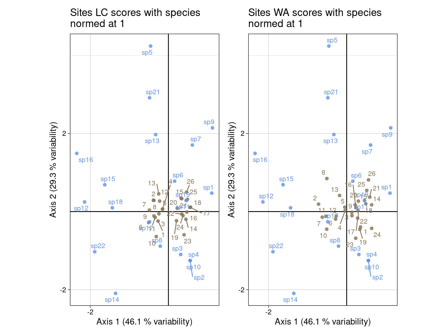
s.corcircle(BS_B1norm,
            labels = colnames(E),
            plabels.col = params$colsite)
s.corcircle(BS_C1norm,
            labels = colnames(T_),
            plabels.col = params$colspp, add = TRUE)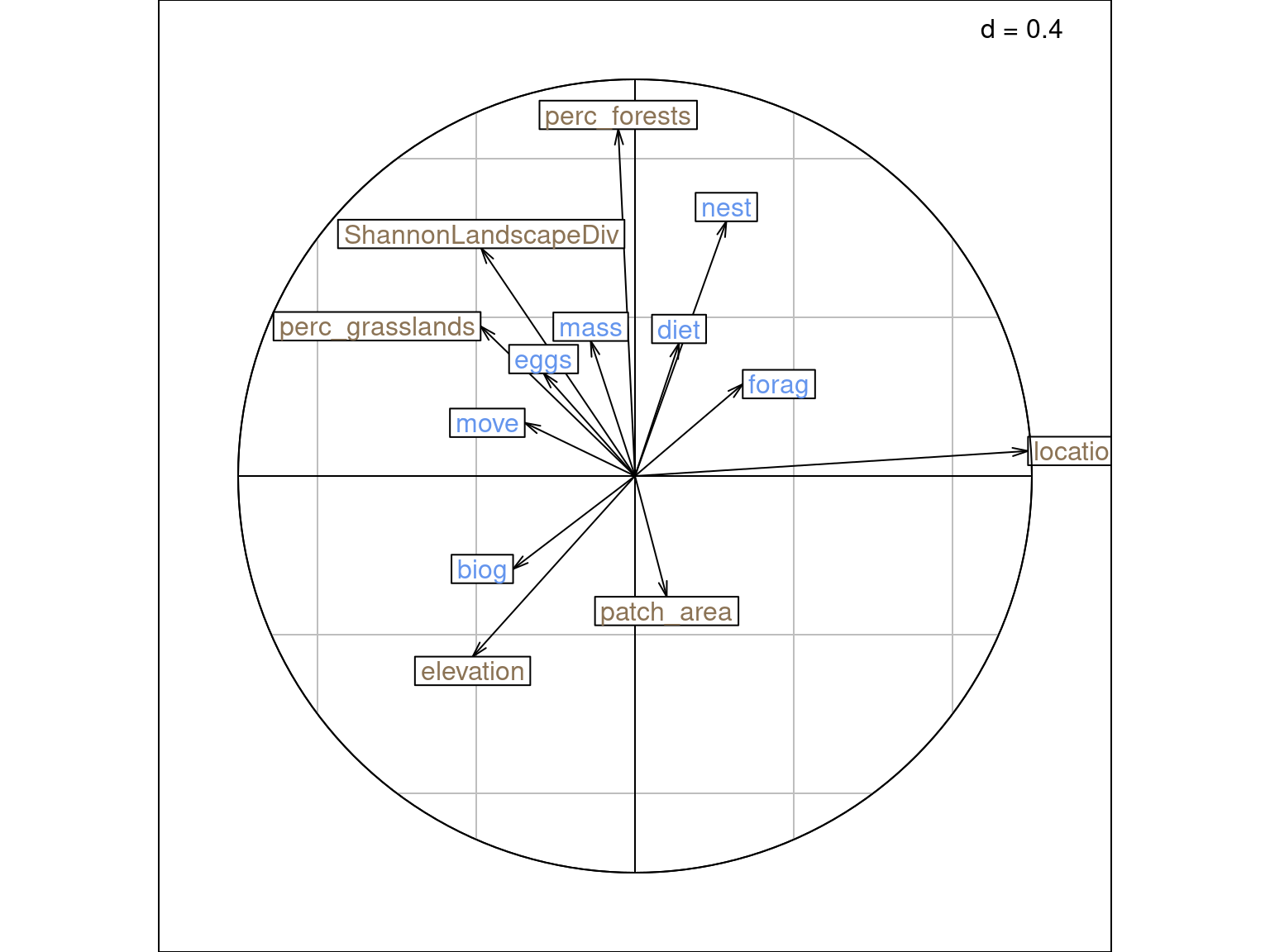
On this plot, we can interpret 5 sets of pairs:
mass and perc_forests is large (arrows size + direction).location variable.The last pair is the individuals on each plot:
Moreover, species traits (\(BS_C^1\)): arrows indicate intra-set correlations.
There is no interpretation for sites - environmental variables (\(U_1\) - \(BS_{B1}\)).
Same plots with ade4:
s.label(dcca$c1, # Species LC1
        plabels.optim = TRUE,
        plabels.col  = params$colspp,
        ppoints.col = params$colspp,
        main = "LC scores for sites")
s.label(dcca$li, # Sites LC
        plabels.optim = TRUE,
        plabels.col  = params$colsite,
        ppoints.col = params$colsite,
        add = TRUE)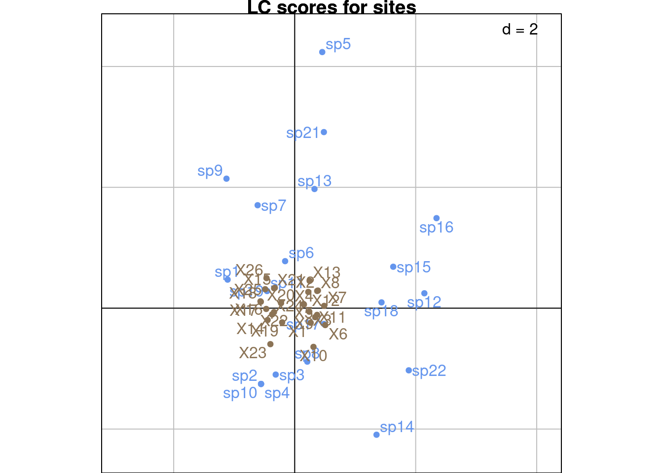
s.label(dcca$c1, # Species LC1
        plabels.optim = TRUE,
        plabels.col  = params$colspp,
        ppoints.col = params$colspp,
        main = "WA scores for sites")
s.label(dcca$lsR, # Sites WA scores
        plabels.optim = TRUE,
        plabels.col  = params$colsite,
        ppoints.col = params$colsite,
        add = TRUE)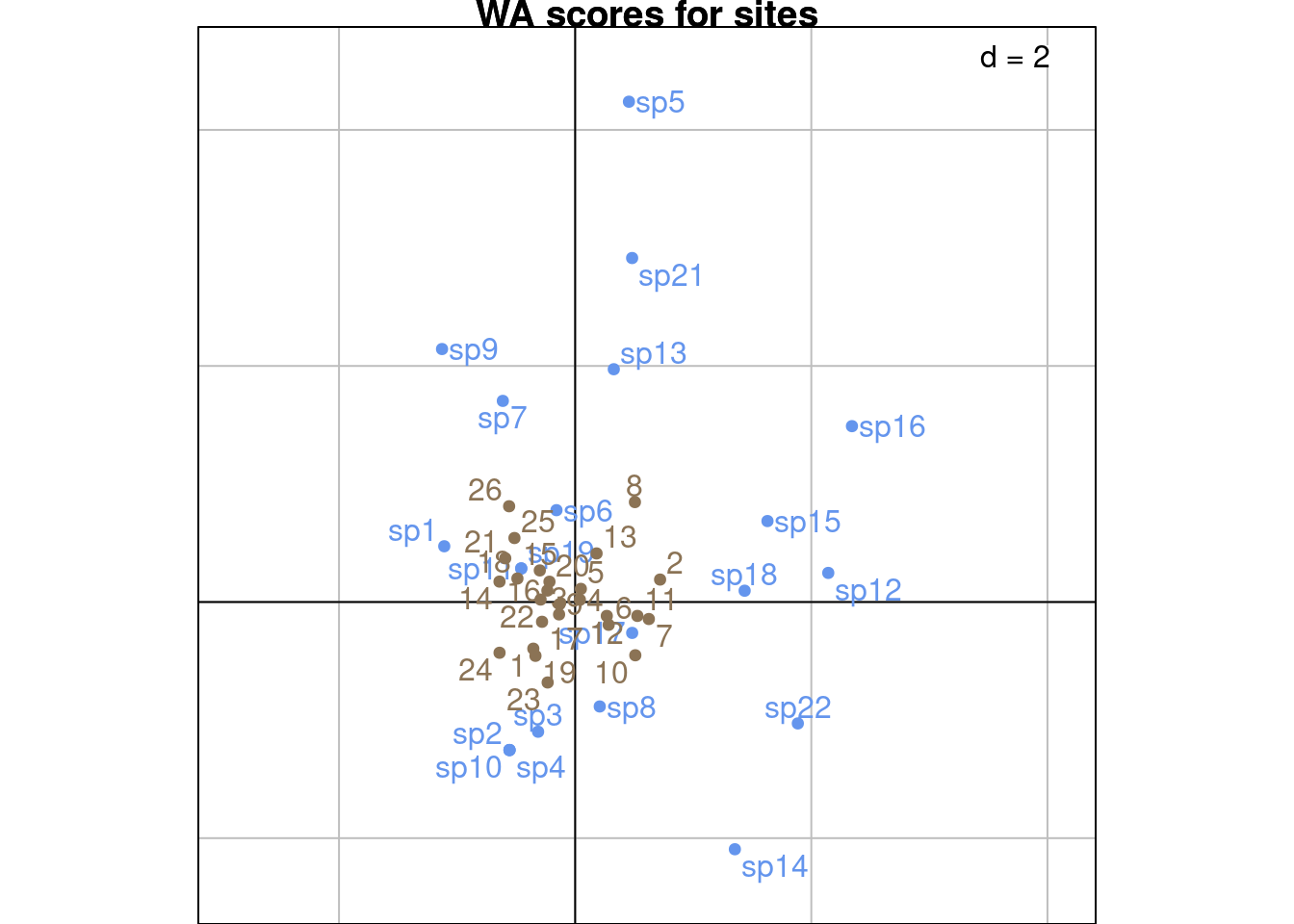
s.corcircle(dcca$corQ,
            plabels.col = params$colspp)
s.corcircle(dcca$corR,
            plabels.col = params$colsite, add = TRUE)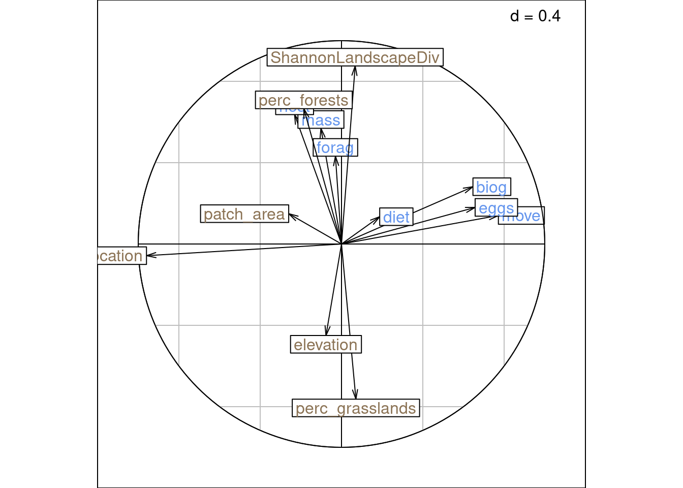
This type of scaling preserves the distances between columns.
With the scaling type 2, \(BS_{B2}\) represents the correlation between environmental variables and sites and \(BS_{C2}\) represents the correlation between species traits and sites.
# LC scores
U2 <- Escaled %*% B # rows
V2 <- Tscaled %*% C %*% Delta # columns

# WA scores
Ustar2 <- solve(Dr) %*% P %*% V2 # rows
Vstar2 <- solve(Dc) %*% t(P) %*% U2 # columns

# Variables scores
BS_B2 <- t(Escaled) %*% Dr %*% U2
# BS_B2 <- B
# BS_C2 <- C %*% Delta
#
# # Normalize
# BS_B2norm <- normalize(BS_B2, 1)
# BS_C2norm <- normalize(BS_C2, 1)all(abs(U2/dcca$l1) - 1 < zero) # LC sites[1] TRUEall(abs(V2/dcca$co) - 1 < zero) # LC spp[1] TRUEall(abs(Vstar2/dcca$lsQ) - 1 < zero) # WA spp[1] TRUEall(abs(Ustar2/dcca$lsR) - 1 < zero) # WA site[1] TRUEall(abs(abs(BS_B2/dcca$corR) - 1) < zero)[1] TRUEWe can either plot:
l1) and species as \(V_2\) (co) (left)l1) and species as \(V^\star_2\) (lsQ) (right)# LC scores
glc <- multiplot(indiv_row = U2, indiv_col = V2,
indiv_row_lab = rownames(Y), indiv_col_lab = colnames(Y),
# var_row = BS_B2norm, var_row_lab = colnames(E),
# var_col = BS_C2norm, var_col_lab = colnames(T_),
row_color = params$colsite, col_color = params$colspp,
eig = lambda) +
ggtitle("Species LC scores with sites\nnormed at 1")
# WA scores
gwa <- multiplot(indiv_row = U2, indiv_col = Vstar2,
indiv_row_lab = rownames(Y), indiv_col_lab = colnames(Y),
# var_row = BS_B2norm, var_row_lab = colnames(E),
# var_col = BS_C2norm, var_col_lab = colnames(T_),
row_color = params$colsite, col_color = params$colspp,
eig = lambda) +
ggtitle("Species WA scores with sites\nnormed at 1")
glc + gwa +
plot_layout(axis_titles = "collect")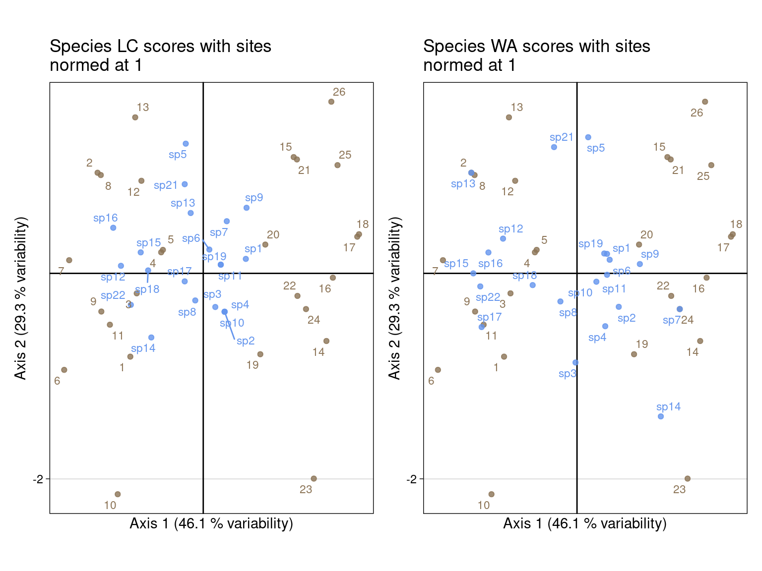
# s.corcircle(BS_B2norm,
#             labels = colnames(E),
#             plabels.col = params$colsite)
# s.corcircle(BS_C2norm,
#             labels = colnames(T_),
#             plabels.col = params$colspp, add = TRUE)
There is no interpretation for species - species traits (\(V_2\) - \(BS_{C2}\)).
With ade4:
s.label(dcca$li, # LC1 sites
        plabels.optim = TRUE,
        plabels.col  = params$colsite,
        ppoints.col = params$colsite,
        main = "LC scores for species")
s.label(dcca$co, # LC species
        plabels.optim = TRUE,
        plabels.col  = params$colspp,
        ppoints.col = params$colspp,
        add = TRUE)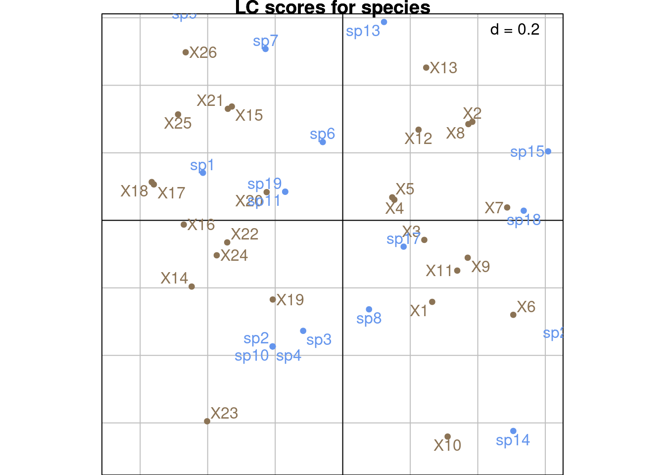
s.label(dcca$l1, # LC1 sites
        plabels.optim = TRUE,
        plabels.col  = params$colsite,
        ppoints.col = params$colsite,
        main = "WA scores for species")
s.label(dcca$lsQ, # WA species
        plabels.optim = TRUE,
        plabels.col  = params$colspp,
        ppoints.col = params$colspp,
        add = TRUE)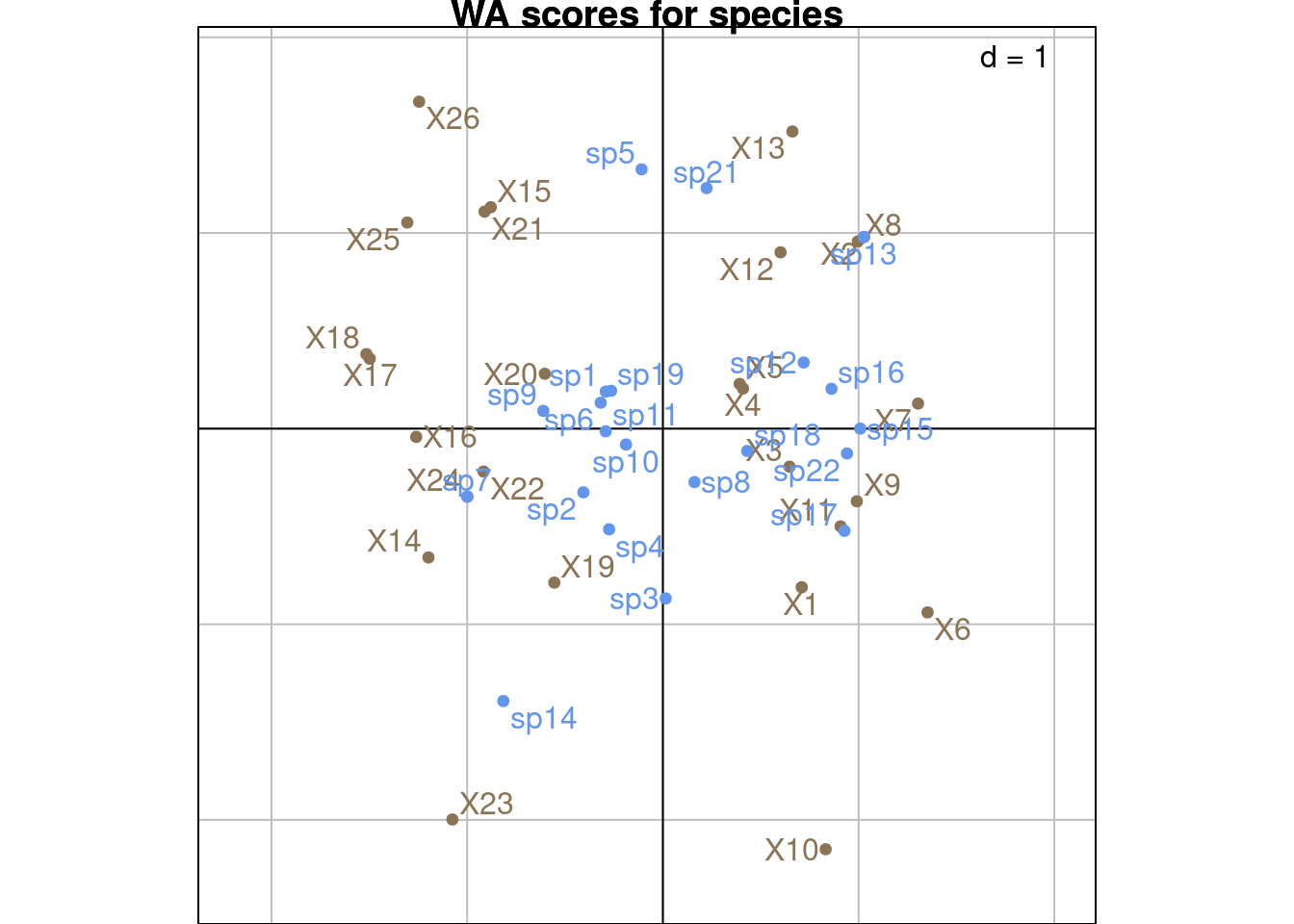
This type of scaling is an intermediate between scalings 1 and 2.
With the scaling type 3, \(BS_{B3}\) and \(BS_{C3}\) represent the geometric mean of their correlation with species and sites.
# LC scores
U3 <- Escaled %*% B %*% Delta^(1/2) # rows
V3 <- Tscaled %*% C %*% Delta^(1/2) # columns

# WA scores
Ustar3 <- solve(Dr) %*% P %*% V3 # rows
Vstar3 <- solve(Dc) %*% t(P) %*% U3 # columns

# Variables scores
BS_B3 <- B %*% Delta^(1/2)
BS_C3 <- C %*% Delta^(1/2)

# Normalize
BS_B3norm <- normalize(BS_B3, 1)
BS_C3norm <- normalize(BS_C3, 1)# LC scores
glc <- multiplot(indiv_row = U3, indiv_col = V3,
indiv_row_lab = rownames(Y), indiv_col_lab = colnames(Y),
# var_row = BS_B3norm, var_row_lab = colnames(E),
# var_col = BS_C3norm, var_col_lab = colnames(T_),
row_color = params$colsite, col_color = params$colspp,
eig = lambda) +
ggtitle("LC scores")
# WA scores
gwa <- multiplot(indiv_row = Ustar3, indiv_col = Vstar3,
indiv_row_lab = rownames(Y), indiv_col_lab = colnames(Y),
# var_row = BS_B3norm, var_row_lab = colnames(E),
# var_col = BS_C3norm, var_col_lab = colnames(T_),
row_color = params$colsite, col_color = params$colspp,
eig = lambda) +
ggtitle("WA scores")
glc + gwa +
plot_layout(axis_titles = "collect")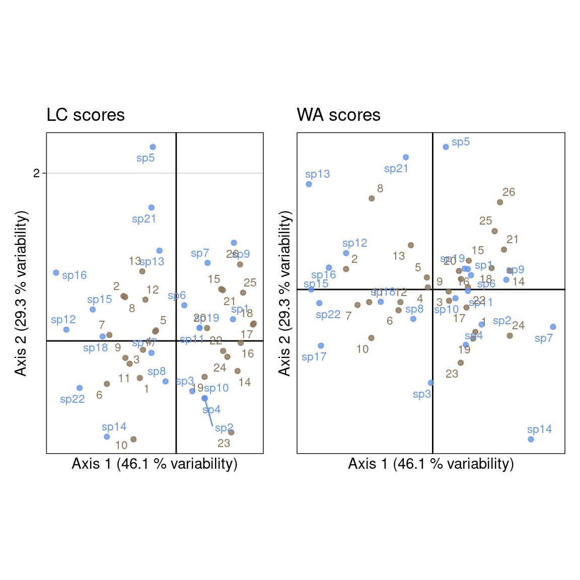
s.corcircle(BS_B3norm,
            labels = colnames(E),
            plabels.col = params$colsite)
s.corcircle(BS_C3norm,
            labels = colnames(T_),
            plabels.col = params$colspp, add = TRUE)
This method finds the linear correlation of row explanatory variables (environmental variables) and the linear correlation of columns explanatory variables (species traits) that maximizes the fourth-corner correlation, i.e. the correlation between these linear combinations of row and columns-variables.
There are other related methods, that have been better described and also more used in ecology: RLQ, community weighted means RDA (CMW-RDA).
Contrary to RLQ, dc-CA takes into account the correlation between the row and column variables. Thus, while RLQ can analyze any number of row and column variables, it is not the case with dc-CA the number of row and column variables must not be large compared to the number of rows/columns in the tables. Also, dc-CA maximizes correlation and RLQ maximizes covariance (Braak, Šmilauer, and Dray 2018).
The eigenvalues of dc-CA are the squares of the fourth-corner correlations.