Reciprocal scaling with CCA

Code

# Paths
library(here)

# Multivariate analysis
library(ade4)
library(adegraphics)

# Matrix algebra
library(expm)

# Plots
library(CAnetwork)

Code

# Define bound for comparison to zero
zero <- 10e-10

Introduction

This is an extension of reciprocal scaling defined for correspondence analysis by Thioulouse and Chessel (1992) to canonical correspondence analysis.

Here, we start from two matrices:

A data matrix $Y$ ($r \times c$)
A matrix of predictor variables (environmental variabnes) $E$ ($r \times l$)

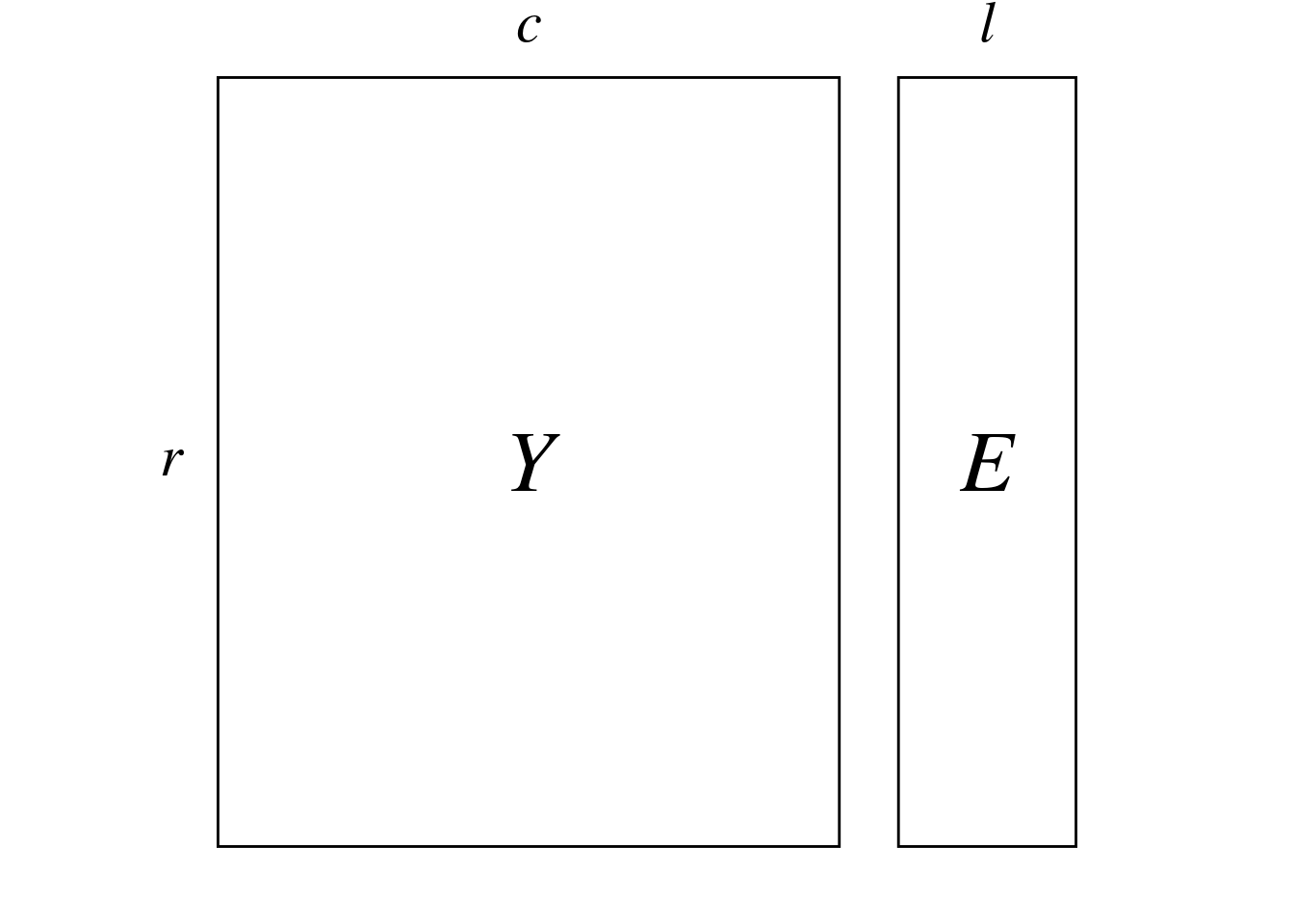
(r <- dim(Y)[1])

[1] 26

(c <- dim(Y)[2])

[1] 21

(l <- ncol(E))

[1] 6

Computation

TL;DR

We can compute reciprocal scaling score using CCorA and CCA scores.

From canonical correlation analysis We perform the CCorA of tables $E_{infl}$ and $Y_{infl}$. The two sets of scores give the correspondences in sites and species space.

From CCA We can show that$scoreC = V$ (c1) and $scoreR = Z2$ (l1).

From canonical correlation analysis

To perform the canonical correlation analysis, we compute the inflated tables $R$ ($n_{\bar{0}} \times l$) and $C$ ($n_{\bar{0}} \times c$) from $Y$ ($r \times c$) and $E$ ($r \times l$). The difference with CA is that we use $E$ instead of $Y$ to compute the inflated table $R$. $R$ is equivalent to $E$ where rows of $E$ are duplicated as many times as there are correspondences in $Y$.

# Transform matrix to count table
P <- Y/sum(Y)
Pfreq <- as.data.frame(as.table(P))
colnames(Pfreq) <- c("row", "col", "Freq")

# Remove the cells with no observation
Pfreq0 <- Pfreq[-which(Pfreq$Freq == 0),]
Pfreq0$colind <- match(Pfreq0$col, colnames(Y)) # match index and species names
Pfreq0$col <- factor(Pfreq0$col)
Pfreq0$row <- factor(Pfreq0$row)

pi_ <- rowSums(P)
p_j <- colSums(P)

We take the frequency table defined before and use it to compute the inflated tables (with weights):

# Create indicator tables
tabR <- acm.disjonctif(as.data.frame(Pfreq0$row))
tabR <- as.matrix(tabR) %*% as.matrix(E) # duplicate rows of E according to the correspondences of Y
tabC <- acm.disjonctif(as.data.frame(Pfreq0$col))
colnames(tabC) <- colnames(Y)

# Get weights
wt <- Pfreq0$Freq

Below are the first lines of tables $R$ and $C$:

Code

knitr::kable(head(tabR, 30))

location	elevation	patch_area	perc_forests	perc_grasslands	ShannonLandscapeDiv
0	10	6.28	7.7882	67.7785	0.232
0	30	7.92	16.4129	43.4066	0.274
0	430	83.24	24.4526	28.4995	0.274
0	420	140.83	41.9966	34.2412	0.260
0	400	140.83	41.9966	34.2412	0.260
0	500	0.50	7.5445	67.0780	0.240
0	470	7.84	19.3087	56.4031	0.253
0	110	21.15	23.4668	49.8908	0.262
0	460	24.82	21.3932	57.0430	0.243
0	450	3.11	4.8285	73.7518	0.216
0	40	6.66	7.4729	66.0061	0.240
0	160	5.63	32.3516	45.0477	0.253
0	160	10.99	29.7139	18.8270	0.291
1	10	6.28	7.7882	67.7785	0.232
1	30	7.92	16.4129	43.4066	0.274
1	430	83.24	24.4526	28.4995	0.274
1	420	140.83	41.9966	34.2412	0.260
1	400	140.83	41.9966	34.2412	0.260
1	500	0.50	7.5445	67.0780	0.240
1	470	7.84	19.3087	56.4031	0.253
1	110	21.15	23.4668	49.8908	0.262
1	460	24.82	21.3932	57.0430	0.243
1	450	3.11	4.8285	73.7518	0.216
1	40	6.66	7.4729	66.0061	0.240
1	160	5.63	32.3516	45.0477	0.253
1	160	10.99	29.7139	18.8270	0.291
0	160	10.99	29.7139	18.8270	0.291
1	500	0.50	7.5445	67.0780	0.240
1	460	24.82	21.3932	57.0430	0.243
1	450	3.11	4.8285	73.7518	0.216

Code

knitr::kable(head(tabC, 30))

sp1	sp2	sp3	sp4	sp5	sp6	sp7	sp8	sp9	sp10	sp11	sp12	sp13	sp14	sp15	sp16	sp17	sp18	sp19	sp21	sp22
1	0	0	0	0	0	0	0	0	0	0	0	0	0	0	0	0	0	0	0	0
1	0	0	0	0	0	0	0	0	0	0	0	0	0	0	0	0	0	0	0	0
1	0	0	0	0	0	0	0	0	0	0	0	0	0	0	0	0	0	0	0	0
1	0	0	0	0	0	0	0	0	0	0	0	0	0	0	0	0	0	0	0	0
1	0	0	0	0	0	0	0	0	0	0	0	0	0	0	0	0	0	0	0	0
1	0	0	0	0	0	0	0	0	0	0	0	0	0	0	0	0	0	0	0	0
1	0	0	0	0	0	0	0	0	0	0	0	0	0	0	0	0	0	0	0	0
1	0	0	0	0	0	0	0	0	0	0	0	0	0	0	0	0	0	0	0	0
1	0	0	0	0	0	0	0	0	0	0	0	0	0	0	0	0	0	0	0	0
1	0	0	0	0	0	0	0	0	0	0	0	0	0	0	0	0	0	0	0	0
1	0	0	0	0	0	0	0	0	0	0	0	0	0	0	0	0	0	0	0	0
1	0	0	0	0	0	0	0	0	0	0	0	0	0	0	0	0	0	0	0	0
1	0	0	0	0	0	0	0	0	0	0	0	0	0	0	0	0	0	0	0	0
1	0	0	0	0	0	0	0	0	0	0	0	0	0	0	0	0	0	0	0	0
1	0	0	0	0	0	0	0	0	0	0	0	0	0	0	0	0	0	0	0	0
1	0	0	0	0	0	0	0	0	0	0	0	0	0	0	0	0	0	0	0	0
1	0	0	0	0	0	0	0	0	0	0	0	0	0	0	0	0	0	0	0	0
1	0	0	0	0	0	0	0	0	0	0	0	0	0	0	0	0	0	0	0	0
1	0	0	0	0	0	0	0	0	0	0	0	0	0	0	0	0	0	0	0	0
1	0	0	0	0	0	0	0	0	0	0	0	0	0	0	0	0	0	0	0	0
1	0	0	0	0	0	0	0	0	0	0	0	0	0	0	0	0	0	0	0	0
1	0	0	0	0	0	0	0	0	0	0	0	0	0	0	0	0	0	0	0	0
1	0	0	0	0	0	0	0	0	0	0	0	0	0	0	0	0	0	0	0	0
1	0	0	0	0	0	0	0	0	0	0	0	0	0	0	0	0	0	0	0	0
1	0	0	0	0	0	0	0	0	0	0	0	0	0	0	0	0	0	0	0	0
1	0	0	0	0	0	0	0	0	0	0	0	0	0	0	0	0	0	0	0	0
0	1	0	0	0	0	0	0	0	0	0	0	0	0	0	0	0	0	0	0	0
0	1	0	0	0	0	0	0	0	0	0	0	0	0	0	0	0	0	0	0	0
0	1	0	0	0	0	0	0	0	0	0	0	0	0	0	0	0	0	0	0	0
0	1	0	0	0	0	0	0	0	0	0	0	0	0	0	0	0	0	0	0	0

Then, we perform a canonical correlation on the scaled tables $R_{scaled}$ and $C_{scaled}$. We find the coefficients $\rho$ and $\gamma$ maximizing the correlation between the scores $S_R = R_{scaled} \rho$ and $S_C = C_{scaled} \gamma$.

# Center tables
tabR_scaled <- scalewt(tabR, wt, 
                       scale = FALSE)
tabC_scaled <- scalewt(tabC, wt, 
                       scale = FALSE)

res <- cancor(diag(sqrt(wt)) %*% tabR_scaled, 
              diag(sqrt(wt)) %*% tabC_scaled, 
              xcenter = FALSE, ycenter = FALSE)
# res gives the coefficients of the linear combinations that maximizes the correlation between the 2 dimensions
dim(res$xcoef) # l columns -> R_scaled is of full rank

[1] 6 6

dim(res$ycoef) # c-1 columns -> C_scaled is not of full rank

[1] 20 20

# Compute these scores from this coef
scoreR <- tabR_scaled[, 1:l]  %*% res$xcoef
scoreC <- tabC_scaled[, 1:(c-1)]  %*% res$ycoef
rownames(scoreC) <- Pfreq0$col
rownames(scoreR) <- Pfreq0$row

From CCA scores

neig <- min(c(r-1, c, l))
ca <- dudi.coa(Y, 
               nf = c-1, 
               scannf = FALSE)
cca <- pcaiv(dudi = ca, 
             df = E,
             scannf = FALSE,
             nf = neig)

sqrt(cca$eig)/res$cor

[1] 1 1 1 1 1 1

We check that unique scores correspond:

fac <- Pfreq0$col
s.class(scoreC,
        wt = wt,
        fac = fac,
        plabels.col = params$colspp, 
        main = "Unique C scores")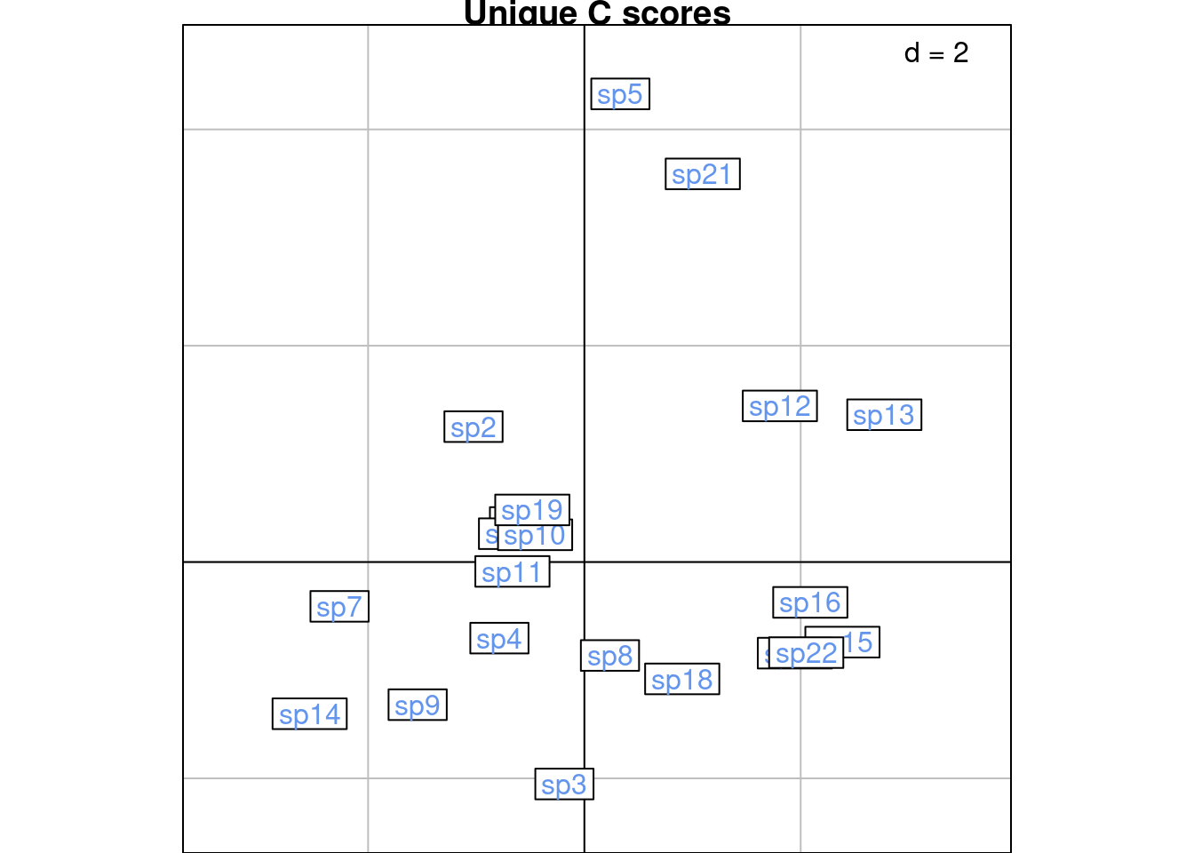

fac <- Pfreq0$row
s.class(scoreR,
        wt = wt,
        fac = fac,
        plabels.col = params$colsite, 
        main = "Unique R scores")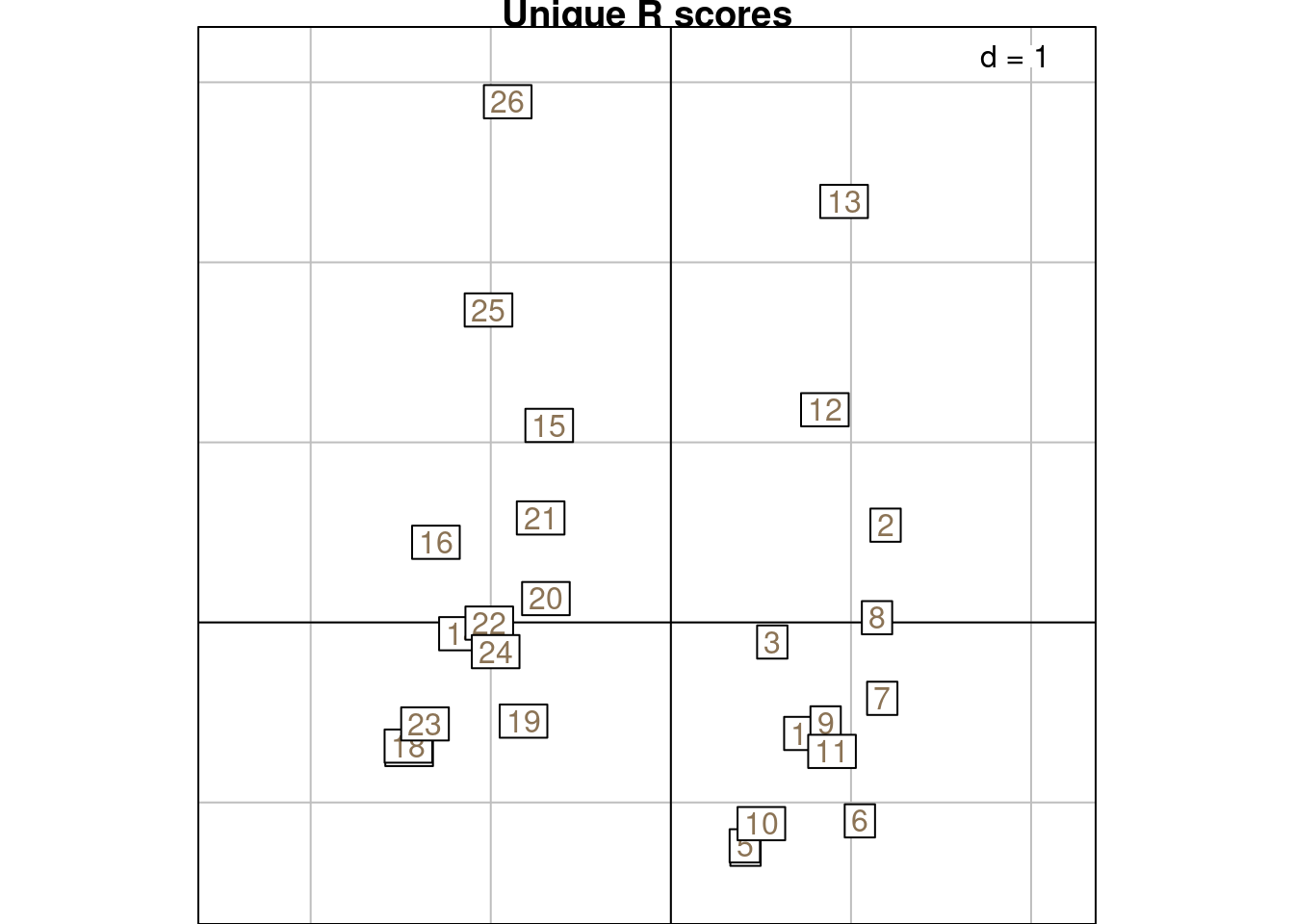

mrowsC <- meanfacwt(scoreC, fac = Pfreq0$col, wt = Pfreq0$Freq)
all(abs(abs(mrowsC/cca$c1) - 1) < zero)

[1] TRUE

mrowsR <- meanfacwt(scoreR, fac = Pfreq0$row, wt = Pfreq0$Freq)
all(abs(abs(mrowsR/cca$l1) - 1) < zero)

[1] TRUE

Conditional means and variances

TL;DR

For the scores computed with R scores and C scores, we have 3 types of formulas:

definition (weighted mean/variance/covariance)
formulas using the CCA scores

Here, we don’t show the definition.

Formulas using CCA scores

using R score

	Rows (sites)	Columns (species)
Mean for axis $k$	$m_k(i) = z2_{ik}$ (`$l1`)	$m_k(j) = v_{jk}$ (`$c1`)
Variance for axis $k$	None	\[s_{jk}^2 = \frac{1}{p_{\cdot j}} \sum_{i = 1}^r \left(p_{ij} {z2_{ik}}^2 - {v_{jk}}^2 \right)\]
Covariance between axes $k$, $l$

using C score

	Rows (sites)	Columns (species)
Mean for axis $k$	$u^\star_{ik}$ (WA score `ls`)	\[v_{jk}\] (`$c1`)
Variance for axis $k$	\[s_k^2(i) = \frac{1}{p_{i \cdot}} \sum_{j = 1}^c \left(p_{ij} v_{jk} \right) - {u^\star_{ik}}^2\]	None
Covariance between axes $k$, $l$

For rows = sites (group per row)

In this section, we compute means and variances per row (for sites).

scoreC

Below is a graphical illustration of scoreC grouped by rows:

s.class(scoreC,
        wt = Pfreq0$Freq,
        fac = as.factor(Pfreq0$row),
        ppoints.col = params$colspp,
        plabels.col = params$colsite, 
        main = "With C score (points = species scores)")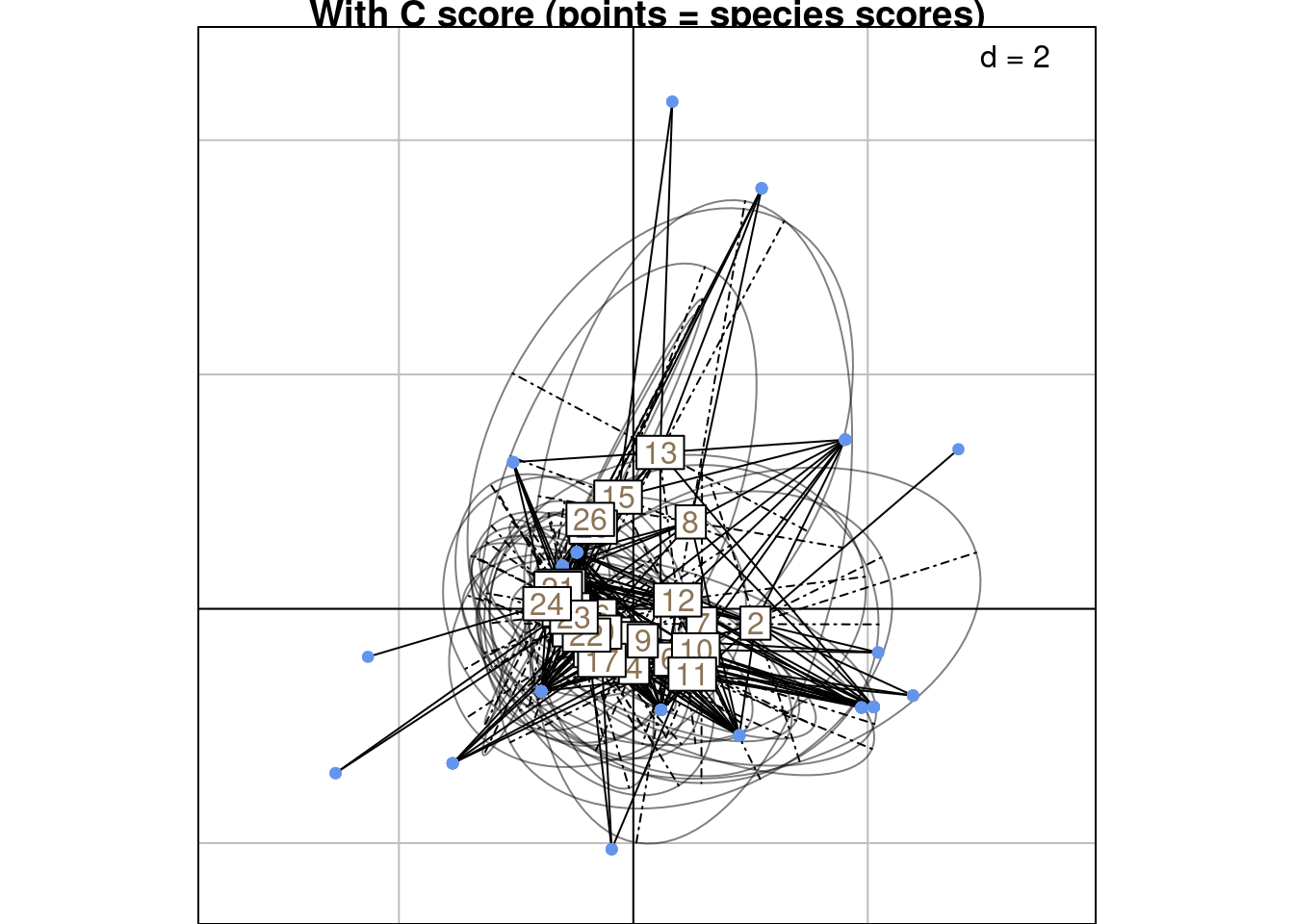

We compute the following mean: $m_k(i) = \frac{1}{y_{i\cdot}} \sum_{j = 1}^c p_{ij} \text{scoreC}_k(i,j)$. To compute these conditional means, we use the meanfacwt function from the ade4 package.

mrowsC <- meanfacwt(scoreC, fac = Pfreq0$row, wt = Pfreq0$Freq)

Then we compare this to a score obtained from CCA.

mrowsC/cca$ls

   Axis1 Axis2 Axis3 Axis4 Axis5 Axis6
1      1     1     1    -1     1     1
2      1     1     1    -1     1     1
3      1     1     1    -1     1     1
4      1     1     1    -1     1     1
5      1     1     1    -1     1     1
6      1     1     1    -1     1     1
7      1     1     1    -1     1     1
8      1     1     1    -1     1     1
9      1     1     1    -1     1     1
10     1     1     1    -1     1     1
11     1     1     1    -1     1     1
12     1     1     1    -1     1     1
13     1     1     1    -1     1     1
14     1     1     1    -1     1     1
15     1     1     1    -1     1     1
16     1     1     1    -1     1     1
17     1     1     1    -1     1     1
18     1     1     1    -1     1     1
19     1     1     1    -1     1     1
20     1     1     1    -1     1     1
21     1     1     1    -1     1     1
22     1     1     1    -1     1     1
23     1     1     1    -1     1     1
24     1     1     1    -1     1     1
25     1     1     1    -1     1     1
26     1     1     1    -1     1     1

??????? axis 4 ?????

Now let’s compute the variance of scoreC per row:

varrowsC <- varfacwt(scoreC, fac = Pfreq0$row, wt = Pfreq0$Freq)

We can use this relationship to find the formula using CCA scores:

varrowsC_CCA <- matrix(nrow = r, 
                       ncol = neig)

for (i in 1:r) {
  # Get CA scores for site i
  Li <- cca$ls[i, ]
  
  # Compute the part with the sum on Cj
  # we add all coordinates Cj^2 weighted by the number of observations on site i
  sumj <- t(P[i, ]) %*% as.matrix(cca$c1)^2
  # sumj <- t(Y[i, ]) %*% as.matrix(cca$co)^2

  # Fill i-th row with site i variance along each axis
  # varrowsC_CCA[i, ] <- 1/(n*lambda_CCA)*((1/pi_[i])*sumj - lambda_CCA*as.numeric(Li)^2)
  varrowsC_CCA[i, ] <- ((1/pi_[i])*sumj - as.numeric(Li)^2)
}

varrowsC[, 1:neig]/varrowsC_CCA

   X1 X2 X3 X4 X5 X6
1   1  1  1  1  1  1
2   1  1  1  1  1  1
3   1  1  1  1  1  1
4   1  1  1  1  1  1
5   1  1  1  1  1  1
6   1  1  1  1  1  1
7   1  1  1  1  1  1
8   1  1  1  1  1  1
9   1  1  1  1  1  1
10  1  1  1  1  1  1
11  1  1  1  1  1  1
12  1  1  1  1  1  1
13  1  1  1  1  1  1
14  1  1  1  1  1  1
15  1  1  1  1  1  1
16  1  1  1  1  1  1
17  1  1  1  1  1  1
18  1  1  1  1  1  1
19  1  1  1  1  1  1
20  1  1  1  1  1  1
21  1  1  1  1  1  1
22  1  1  1  1  1  1
23  1  1  1  1  1  1
24  1  1  1  1  1  1
25  1  1  1  1  1  1
26  1  1  1  1  1  1

varrowsC[, 1:neig]/varrowsC_CCA

   X1 X2 X3 X4 X5 X6
1   1  1  1  1  1  1
2   1  1  1  1  1  1
3   1  1  1  1  1  1
4   1  1  1  1  1  1
5   1  1  1  1  1  1
6   1  1  1  1  1  1
7   1  1  1  1  1  1
8   1  1  1  1  1  1
9   1  1  1  1  1  1
10  1  1  1  1  1  1
11  1  1  1  1  1  1
12  1  1  1  1  1  1
13  1  1  1  1  1  1
14  1  1  1  1  1  1
15  1  1  1  1  1  1
16  1  1  1  1  1  1
17  1  1  1  1  1  1
18  1  1  1  1  1  1
19  1  1  1  1  1  1
20  1  1  1  1  1  1
21  1  1  1  1  1  1
22  1  1  1  1  1  1
23  1  1  1  1  1  1
24  1  1  1  1  1  1
25  1  1  1  1  1  1
26  1  1  1  1  1  1

We can also compute the covariance between axes $k$ and $l$ for site $i$ from CCorA scores:

\[c_{kl}(i) = \frac{1}{y_{i+}}\sum_{j=1}^c p_{ij}{s_Y}_k(i, j){s_Y}_l(i, j) - m_{ik}m_{il}\]

covarrowsC <- covfacwt(scoreC, fac = Pfreq0$row, wt = Pfreq0$Freq)

This is equivalent to the following formula using CCA scores:

\[ c_{kl}(i) = \frac{1}{n} \left( \sum_{j=1}^c p_{ij}v_{jk}v_{jl} - u^\star_{ik}u^\star_{il} \right)\]

# Define axes k and l
kk <- 1
lk <- 2

Below, we compute the covariance for all resources between axes $k=$1 and $l = $2 and compare to the covariance computed from the weighted covariance of CCorA scores:

# Initialize vector
covarrowsC_CCA <- vector(mode = "numeric", length = r)

for (i in 1:r) {
  # Compute the sum
  sumj <- sum(P[i, ]*cca$c1[, kk]*cca$c1[, lk])

  # Covariance for species i
  covarrowsC_CCA[i] <- ((1/pi_[i])*sumj - cca$ls[i, kk]*cca$ls[i, lk])
}

covarrowsC_kl <- sapply(covarrowsC, function(x) x[kk, lk])
res <- covarrowsC_CCA/covarrowsC_kl
all(abs(abs(res) - 1) < zero)

[1] TRUE

scoreR

Now, we compute the mean per row (site) from the row (sites) scores.

Below is a graphical illustration of scoreR grouped by rows:

s.class(scoreR,
        wt = Pfreq0$Freq,
        fac = as.factor(Pfreq0$row),
        ppoints.col = params$colsite,
        plabels.col = params$colsite, 
        main = "With R score (points = sites scores)")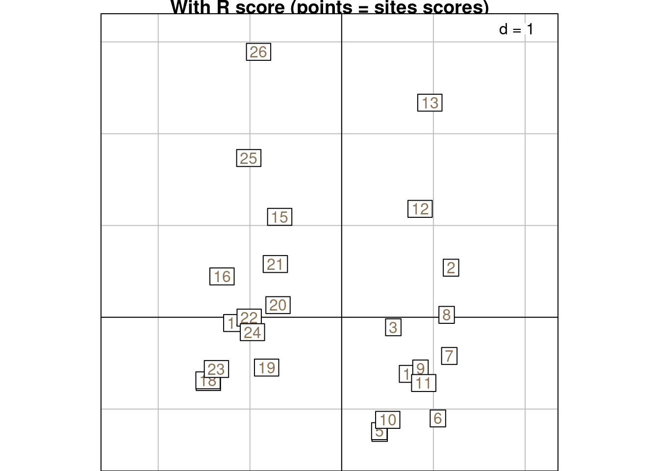

All points of the same site ares superimposed.

mrowsR <- meanfacwt(scoreR, fac = Pfreq0$row, wt = Pfreq0$Freq)

mrowsR/cca$l1

   RS1 RS2 RS3 RS4 RS5 RS6
1    1   1   1  -1   1   1
2    1   1   1  -1   1   1
3    1   1   1  -1   1   1
4    1   1   1  -1   1   1
5    1   1   1  -1   1   1
6    1   1   1  -1   1   1
7    1   1   1  -1   1   1
8    1   1   1  -1   1   1
9    1   1   1  -1   1   1
10   1   1   1  -1   1   1
11   1   1   1  -1   1   1
12   1   1   1  -1   1   1
13   1   1   1  -1   1   1
14   1   1   1  -1   1   1
15   1   1   1  -1   1   1
16   1   1   1  -1   1   1
17   1   1   1  -1   1   1
18   1   1   1  -1   1   1
19   1   1   1  -1   1   1
20   1   1   1  -1   1   1
21   1   1   1  -1   1   1
22   1   1   1  -1   1   1
23   1   1   1  -1   1   1
24   1   1   1  -1   1   1
25   1   1   1  -1   1   1
26   1   1   1  -1   1   1

The variance is null.

For columns = species (group per column)

scoreC

We group the scoreC per species. Below is an illustration:

s.class(scoreC,
        wt = Pfreq0$Freq,
        fac = as.factor(Pfreq0$colind),
        lab = colnames(Y),
        ppoints.col = params$colspp,
        plabels.col = params$colspp, 
        main = "With C score (points = species scores)")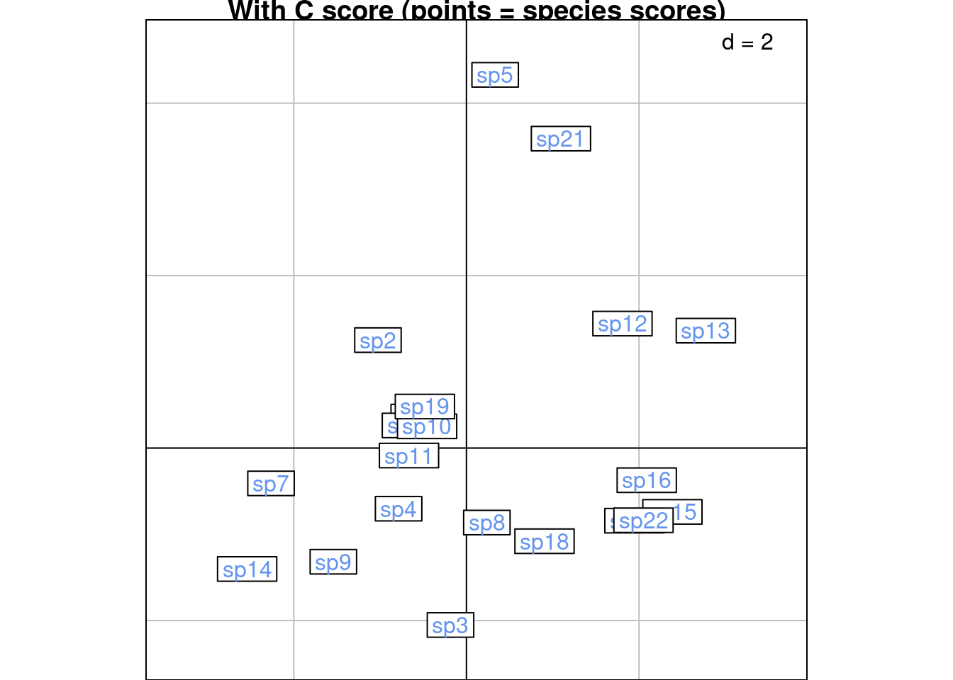

mcolsC <- meanfacwt(scoreC, fac = Pfreq0$colind, wt = Pfreq0$Freq)

mcolsC/cca$c1

     CS1 CS2 CS3 CS4 CS5 CS6
sp1    1   1   1  -1   1   1
sp2    1   1   1  -1   1   1
sp3    1   1   1  -1   1   1
sp4    1   1   1  -1   1   1
sp5    1   1   1  -1   1   1
sp6    1   1   1  -1   1   1
sp7    1   1   1  -1   1   1
sp8    1   1   1  -1   1   1
sp9    1   1   1  -1   1   1
sp10   1   1   1  -1   1   1
sp11   1   1   1  -1   1   1
sp12   1   1   1  -1   1   1
sp13   1   1   1  -1   1   1
sp14   1   1   1  -1   1   1
sp15   1   1   1  -1   1   1
sp16   1   1   1  -1   1   1
sp17   1   1   1  -1   1   1
sp18   1   1   1  -1   1   1
sp19   1   1   1  -1   1   1
sp21   1   1   1  -1   1   1
sp22   1   1   1  -1   1   1

The variance is null.

scoreR

Below are the scoreR grouped by column:

s.class(scoreR,
        wt = Pfreq0$Freq,
        fac = as.factor(Pfreq0$colind),
        lab = colnames(Y),
        ppoints.col = params$colsite,
        plabels.col = params$colspp, 
        main = "With R score (points = sites scores)")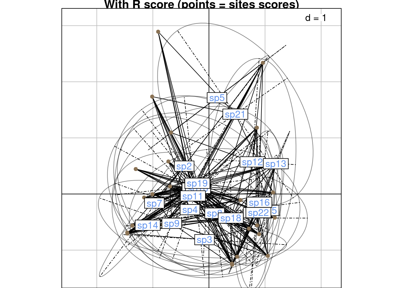

mcolsR <- meanfacwt(scoreR, fac = Pfreq0$colind, wt = Pfreq0$Freq)

mcolsR/cca$co

     Comp1 Comp2 Comp3 Comp4 Comp5 Comp6
sp1      1     1     1    -1     1     1
sp2      1     1     1    -1     1     1
sp3      1     1     1    -1     1     1
sp4      1     1     1    -1     1     1
sp5      1     1     1    -1     1     1
sp6      1     1     1    -1     1     1
sp7      1     1     1    -1     1     1
sp8      1     1     1    -1     1     1
sp9      1     1     1    -1     1     1
sp10     1     1     1    -1     1     1
sp11     1     1     1    -1     1     1
sp12     1     1     1    -1     1     1
sp13     1     1     1    -1     1     1
sp14     1     1     1    -1     1     1
sp15     1     1     1    -1     1     1
sp16     1     1     1    -1     1     1
sp17     1     1     1    -1     1     1
sp18     1     1     1    -1     1     1
sp19     1     1     1    -1     1     1
sp21     1     1     1    -1     1     1
sp22     1     1     1    -1     1     1

varcolsR <- varfacwt(scoreR, fac = Pfreq0$colind, wt = Pfreq0$Freq)

Similarly we can use this relationship to compute the variance directly from the CCA scores (see in table).

We can also compute the covariance between axes $k$ and $l$ for species $j$ from CCorA scores:

\[c_{kl}(j) = \frac{1}{y_{+j}}\sum_{i=1}^r p_{ij}{s_R}_k(i, j){s_R}_l(i, j) - m_{jk}m_{jl}\]

covarcolsR <- covfacwt(scoreR, fac = Pfreq0$col, wt = Pfreq0$Freq)

This is equivalent to the following formula using CCA scores:

\[c_{kl}(j) = \frac{1}{n} \left( \sum_{i=1}^r p_{ij}z2_{ik}z2_{il} - v^\star_{jk}v^\star_{jl} \right)\]

# Define axes k and l
kk <- 1
lk <- 2

Below, we compute the covariance for all resources between axes $k=$1 and $l = $2 and compare to the covariance computed from the weighted covariance of CCorA scores:

# Initialize vector
covarcolsR_CCA <- vector(mode = "numeric", length = c)

for (j in 1:c) {
  # Compute the sum
  sumi <- sum(P[, j]*cca$l1[, kk]*cca$l1[, lk])

  # Covariance for species i
  covarcolsR_CCA[j] <- ((1/p_j[j])*sumi - cca$co[j, kk]*cca$co[j, lk])
}

# Species that appear only once in a site
sp1 <- which(colnames(Y) %in% c("sp7", "sp13"))

covarcolsR_kl <- sapply(covarcolsR, function(x) x[kk, lk])
res <- (covarcolsR_CCA/covarcolsR_kl)[-sp1]
all(abs(abs(res) - 1) < zero)

[1] TRUE

Non-reciprocal score

We can remain in the 2 biplots showing $V$ with $U^\star$ (c1 and ls) (scaling type 1 = rows niches) and $U$ and $V^\star$ (co and l1) (scaling type 2 = column niches).

$H_1$ (scaling type 1, rows niches)

To do that, we define the “CA-correspondences” $h1_k(i, j)$ for scaling type 1:

\[h1_k(i, j) = \frac{u^\star_k(i) + v_k(j)}{2}\]

Code

# Initialize results matrix
H1 <- matrix(nrow = nrow(Pfreq0), 
             ncol = neig)

for (k in 1:neig) { # For each axis
  ind <- 1 # initialize row index
  for (obs in 1:nrow(Pfreq0)) { # For each observation
    i <- Pfreq0$row[obs]
    j <- Pfreq0$col[obs]
    H1[ind, k] <- (cca$ls[i, k] + cca$c1[j, k])/2
    ind <- ind + 1
  }
}

Code

corresp <- paste(Pfreq0$row, Pfreq0$col, sep = "-")
multiplot(indiv_row = as.data.frame(H1), 
          indiv_row_lab = corresp,
          row_color = "black")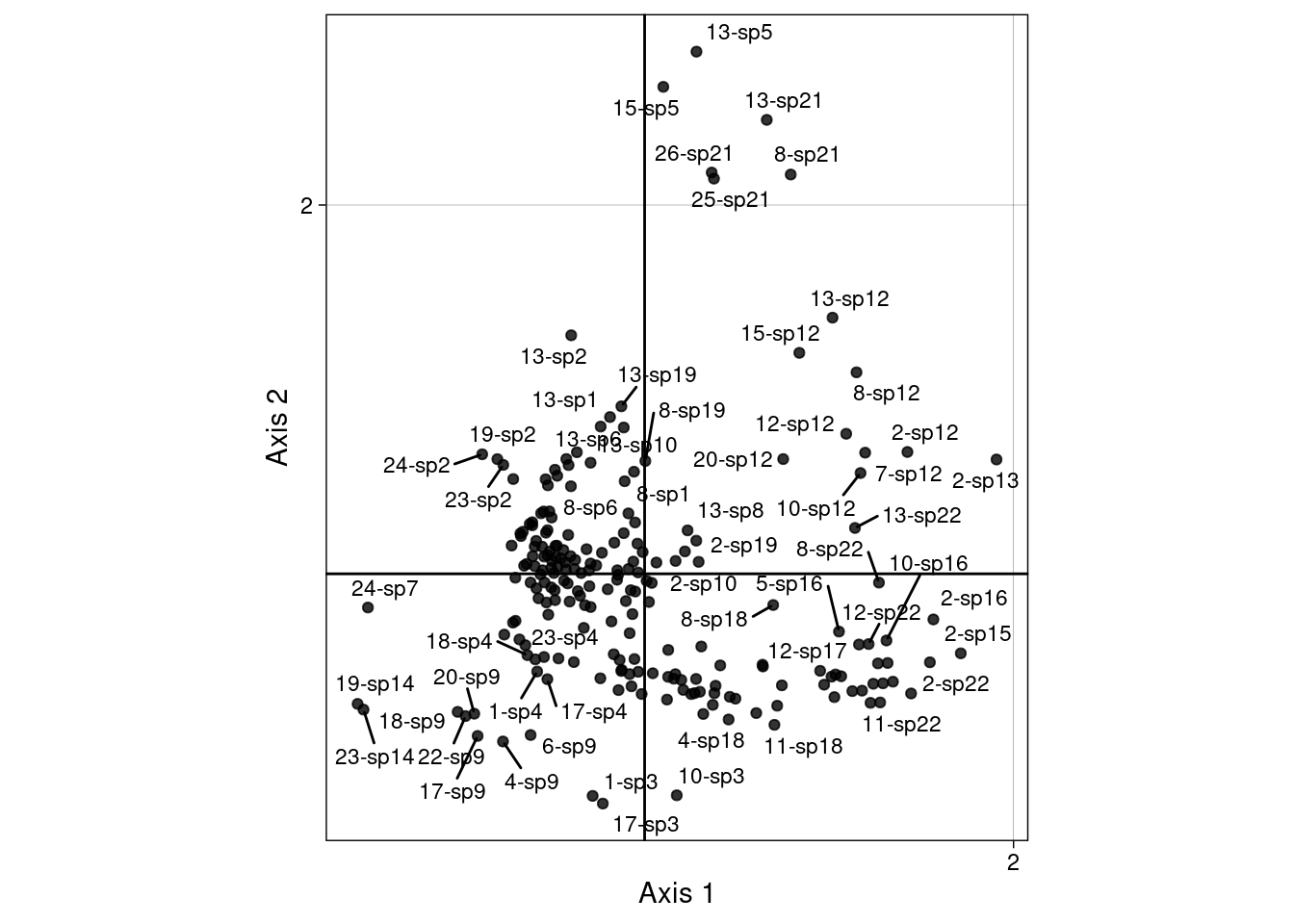

# Groupwise mean
mrows_nr <- meanfacwt(H1, fac = Pfreq0$row, wt = Pfreq0$Freq)
all(abs(abs(mrows_nr/cca$ls) - 1) < zero)

[1] TRUE

# Groupwise variance ---
# Compare to RC score
varrows_nr <- varfacwt(H1, fac = Pfreq0$row, wt = Pfreq0$Freq)
# Compare to mean of scoreC
res <- 4*varrows_nr  # Factor 4
all(abs(abs(res/varrowsC[, 1:neig]) - 1) < zero)

[1] TRUE

# Groupwise covariance
covarrows_nr <- covfacwt(H1, fac = Pfreq0$row, wt = Pfreq0$Freq)
res <- lapply(covarrows_nr, function(x) x*4)  # Factor 4
# We check for the first covariance
all(abs(abs(res[[1]]/covarrowsC[[1]][1:l, 1:l]) - 1) < zero)

[1] TRUE

Code

s.class(H1, 
        fac = Pfreq0$row, plabels.col = params$colsite, 
        wt = Pfreq0$Freq,
        main = "Non-reciprocal scaling")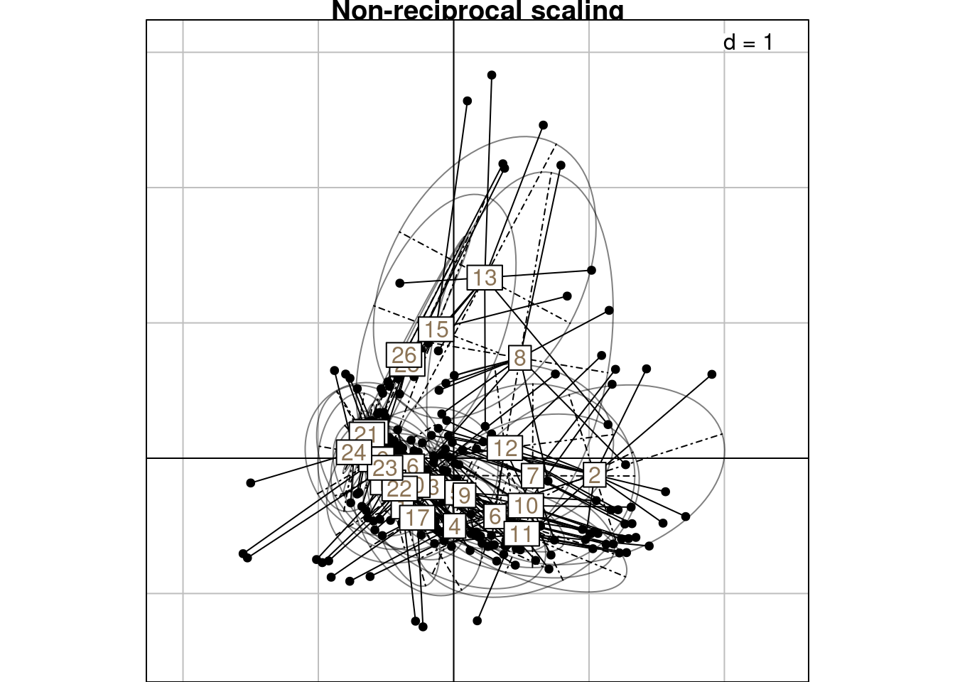

$h1_k(i, j)$ can also be defined from the canonical correlation scores:

\[h1_k(i, j) = \frac{m_{ik} + {s_Y}_k(i, j)}{2}\]

tabR <- as.matrix(acm.disjonctif(as.data.frame(Pfreq0$row)))
scoreRls <- tabR %*% mrowsC # Duplicate means according to correspondences of R

# Find back the formula from the scores 
H1_cancor <- (scoreRls[, 1:l] + scoreC[, 1:l])/2

all(abs(abs(H1_cancor/H1) - 1) < zero)

[1] TRUE

$H_2$ (scaling type 2, columns niches)

We define the “CA-correspondences” $h2_k(i, j)$ for scaling type 2:

\[h2_k(i, j) = \frac{z2_k(i) + v^\star_k(j)}{2}\]

Code

# Initialize results matrix
H2 <- matrix(nrow = nrow(Pfreq0), 
             ncol = neig)

for (k in 1:neig) { # For each axis
  ind <- 1 # initialize row index
  for (obs in 1:nrow(Pfreq0)) { # For each observation
    i <- Pfreq0$row[obs]
    j <- Pfreq0$col[obs]
    H2[ind, k] <- (cca$l1[i, k] + cca$co[j, k])/2
    ind <- ind + 1
  }
}

Code

corresp <- paste(Pfreq0$row, Pfreq0$col, sep = "-")
multiplot(indiv_row = as.data.frame(H2), 
          indiv_row_lab = corresp,
          row_color = "black")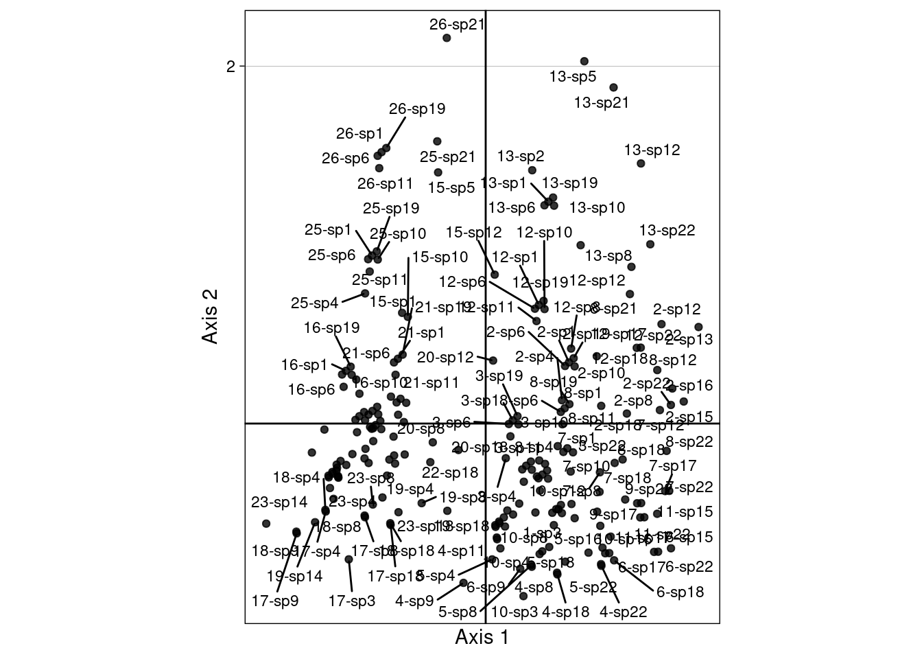

# Groupwise mean ---
mcols_nr <- meanfacwt(H2, fac = Pfreq0$col, wt = Pfreq0$Freq)
# Compare with CCA score
all(abs(abs(mcols_nr/cca$co) - 1) < zero)

[1] TRUE

# Groupwise variance ---
varcols_nr <- varfacwt(H2, fac = Pfreq0$col, wt = Pfreq0$Freq)

Code

fac_col <- factor(Pfreq0$col)
s.class(H2, 
        fac = fac_col, plabels.col = params$colspp, 
        wt = Pfreq0$Freq,
        main = "Non-reciprocal scaling")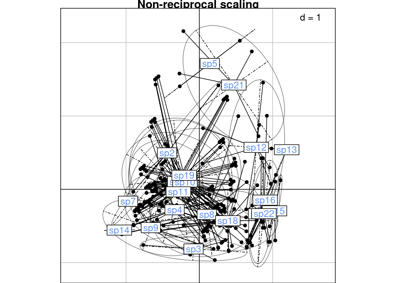

$h2_k(i, j)$ can also be defined from the canonical correlation scores:

\[h2_k(i, j) = \frac{ {s_R}_k(i, j) + {s_Y}_k(i, j) \sqrt{\lambda_k} }{2}\]

# Find back the formula from the scores 
H2_cancor <- (scoreR[, 1:neig] + scoreC[, 1:neig] %*% diag(cca$eig^(1/2)))/2
all(abs(abs(H2_cancor/H2) - 1) < zero)

[1] TRUE

References

Thioulouse, Jean, and Daniel Chessel. 1992. “A Method for Reciprocal Scaling of Species Tolerance and Sample Diversity: Ecological Archives.” Ecology 73 (2): 670–80. https://doi.org/10.2307/1940773.

	Rows (sites)	Columns (species)
Mean for axis \(k\)	\(m_k(i) = z2_{ik}\) (`$l1`)	\(m_k(j) = v_{jk}\) (`$c1`)
Variance for axis \(k\)	None	\[s_{jk}^2 = \frac{1}{p_{\cdot j}} \sum_{i = 1}^r \left(p_{ij} {z2_{ik}}^2 - {v_{jk}}^2 \right)\]
Covariance between axes \(k\), \(l\)

Reciprocal scaling with CCA

Introduction

Computation

From canonical correlation analysis

From CCA scores

Conditional means and variances

For rows = sites (group per row)

scoreC

scoreR

For columns = species (group per column)

scoreC

scoreR

Non-reciprocal score

\(H_1\) (scaling type 1, rows niches)

\(H_2\) (scaling type 2, columns niches)

References