This vignette shows how to compute diversity indices from camera trap data.
Import data
data(mica, package = "camtraptor")
records <- mica$data$observations
Summarize data
To compute diversity indices, we need the number and proportion of
sightings for each species per camera. For that, we use the function
summarize_species with by_cam = TRUE:
spp_cam <- summarize_species(records,
                             spp_col = "vernacularNames.en",
                             cam_col = "deploymentID",
                             obstype_col = "observationType",
                             count_col = "count",
                             by_cam = TRUE,
                             NA_count_placeholder = 1)

knitr::kable(spp_cam)| vernacularNames.en | observationType | deploymentID | sightings | individuals | sightings_prop | individuals_prop |
|---|---|---|---|---|---|---|
| Eurasian beaver | animal | 577b543a-2cf1-4b23-b6d2-cda7e2eac372 | 1 | 1 | 0.1111111 | 0.1111111 |
| European polecat | animal | 577b543a-2cf1-4b23-b6d2-cda7e2eac372 | 3 | 3 | 0.3333333 | 0.3333333 |
| beech marten | animal | 577b543a-2cf1-4b23-b6d2-cda7e2eac372 | 1 | 1 | 0.1111111 | 0.1111111 |
| gadwall | animal | 29b7d356-4bb4-4ec4-b792-2af5cc32efa8 | 3 | 6 | 0.3000000 | 0.2727273 |
| great herons | animal | 62c200a9-0e03-4495-bcd8-032944f6f5a1 | 2 | 2 | 0.4000000 | 0.4000000 |
| grey heron | animal | 62c200a9-0e03-4495-bcd8-032944f6f5a1 | 1 | 1 | 0.2000000 | 0.2000000 |
| human | human | 7ca633fa-64f8-4cfc-a628-6b0c419056d7 | 1 | 2 | 0.3333333 | 0.5000000 |
| mallard | animal | 29b7d356-4bb4-4ec4-b792-2af5cc32efa8 | 4 | 13 | 0.4000000 | 0.5909091 |
| red fox | animal | 577b543a-2cf1-4b23-b6d2-cda7e2eac372 | 1 | 1 | 0.1111111 | 0.1111111 |
| NA | blank | 29b7d356-4bb4-4ec4-b792-2af5cc32efa8 | 1 | 1 | 0.1000000 | 0.0454545 |
| NA | blank | 577b543a-2cf1-4b23-b6d2-cda7e2eac372 | 3 | 3 | 0.3333333 | 0.3333333 |
| NA | unknown | 29b7d356-4bb4-4ec4-b792-2af5cc32efa8 | 2 | 2 | 0.2000000 | 0.0909091 |
| NA | unclassified | 62c200a9-0e03-4495-bcd8-032944f6f5a1 | 2 | 2 | 0.4000000 | 0.4000000 |
| NA | unclassified | 7ca633fa-64f8-4cfc-a628-6b0c419056d7 | 2 | 2 | 0.6666667 | 0.5000000 |
Compute diversity indices
Then, we can compute diversity indices by feeding this summary
dataframe to the get_diversity_indices function.
div <- get_diversity_indices(spp_cam,
                             spp_col = "vernacularNames.en",
                             cam_col = "deploymentID")

knitr::kable(div)| deploymentID | richness | shannon | simpson |
|---|---|---|---|
| 29b7d356-4bb4-4ec4-b792-2af5cc32efa8 | 4 | 1.0237155 | 0.4069264 |
| 577b543a-2cf1-4b23-b6d2-cda7e2eac372 | 5 | 1.4648164 | 0.1666667 |
| 62c200a9-0e03-4495-bcd8-032944f6f5a1 | 3 | 1.0549202 | 0.2000000 |
| 7ca633fa-64f8-4cfc-a628-6b0c419056d7 | 2 | 0.6931472 | 0.3333333 |
Let denote the species and denote the cameras. is the number of species seen at camera . is the total number of individuals of all species seen at a camera . and represent respectively the count and proportion if individuals of species seen at a camera . This function computes:
- richness (the number of species seen at camera ).
- Shannon index . It ranges between 0 and , zero indicating the lowest diversity.
- Simpson index . It ranges between 0 and 1, one indicating the lowest diversity.
Optionally, you can also provide the name of the columns containing
counts and proportions (but they default to the name given by the
summarize_species function).
div <- get_diversity_indices(spp_cam,
                             spp_col = "vernacularNames.en",
                             cam_col = "deploymentID",
                             count_col = "individuals",
                             prop_col = "individuals_prop")
Plot diversity indices
Although it is then simple to use the diversity dataframe to make a
custom plot, the helper function plot_diversity is
provided.
Here, we plot the richness.
plot_diversity(div,
               div_col = "richness",
               cam_col = "deploymentID") +
  ggtitle("Species richness")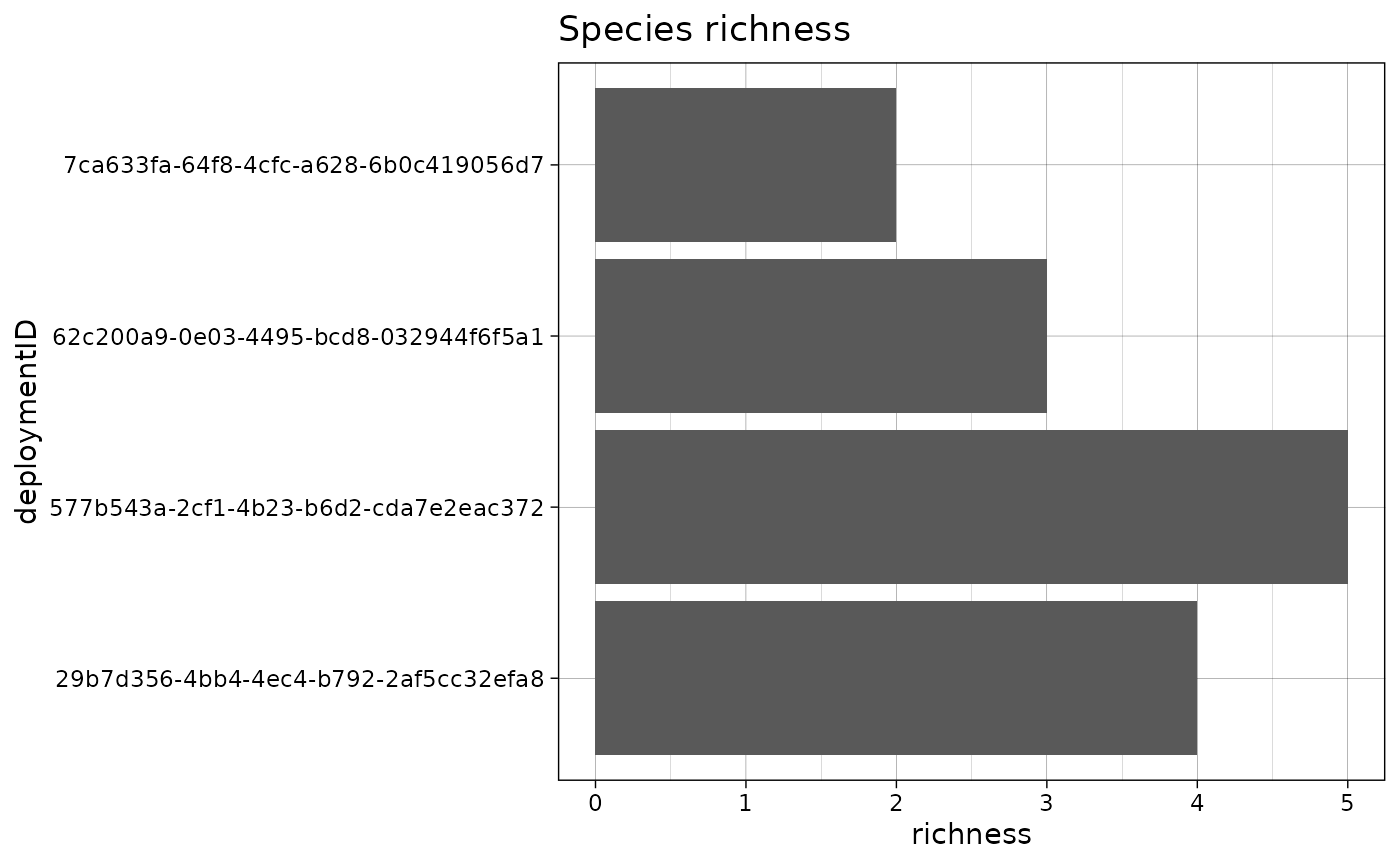
The plot can also be made interactive.
pr <- plot_diversity(div,
                     div_col = "richness",
                     cam_col = "deploymentID",
                     interactive = TRUE) +
  ggtitle("Species richness")

girafe(ggobj = pr)
In case you want to show more cameras than the ones in the
div dataframe, you can use the cam_vec
argument.
div_less <- div[1:3, ]
cameras <- unique(div$deploymentID)

# We deleted one camera
unique(div_less$deploymentID)
#> [1] "29b7d356-4bb4-4ec4-b792-2af5cc32efa8"
#> [2] "577b543a-2cf1-4b23-b6d2-cda7e2eac372"
#> [3] "62c200a9-0e03-4495-bcd8-032944f6f5a1"

# But it is still in cameras
cameras
#> [1] "29b7d356-4bb4-4ec4-b792-2af5cc32efa8"
#> [2] "577b543a-2cf1-4b23-b6d2-cda7e2eac372"
#> [3] "62c200a9-0e03-4495-bcd8-032944f6f5a1"
#> [4] "7ca633fa-64f8-4cfc-a628-6b0c419056d7"
pr <- plot_diversity(div_less,
                     div_col = "richness",
                     cam_col = "deploymentID",
                     cam_vec = cameras,
                     interactive = TRUE) +
  ggtitle("Species richness")

girafe(ggobj = pr)
Finally, by changing the div_col argument you can plot
multiple diversity indices.
ph <- plot_diversity(div,
                     div_col = "shannon",
                     cam_col = "deploymentID",
                     interactive = TRUE) +
  ggtitle("Shannon diversity index")

pd <- plot_diversity(div,
                     div_col = "simpson",
                     cam_col = "deploymentID",
                     interactive = TRUE) +
   ggtitle("Simpson diversity index")

girafe(ggobj = ph)
girafe(ggobj = pd)