set.seed(42)

M <- 100 # Number of sites
p <- 0.4 # Detection probability
psi <- 0.8 # Occupancy

# Simulate a number of visits for each site
nvisit <- rpois(n = M, lambda = 3)
nvisit[nvisit == 0] <- 1 # Don't allow zero visits

# Initialize vectors
z <- vector(mode = "numeric", length = M)
y <- vector(mode = "list", length = M)

for (i in 1:M) { # For each site
  # Simulate true presence/absence at site i
  zi <- rbinom(n = 1, size = 1, prob = psi)

  # Simulate observed presence/absence at site i
  # for all visits
  yij <- rbinom(n = nvisit[i],
                size = 1, prob = p*zi)

  z[i] <- zi # True sites states
  y[[i]] <- yij # Detections
}Present, but not detected

Introduction
- First published by MacKenzie et al. (2002) in the context of species occurrence modelling
- Many extensions: dynamic occupancy (MacKenzie et al. 2003), multiple species (Rota et al. 2016), continuous detection process (MacKenzie et al. 2003)…
- Here: original simple occupancy model
Model
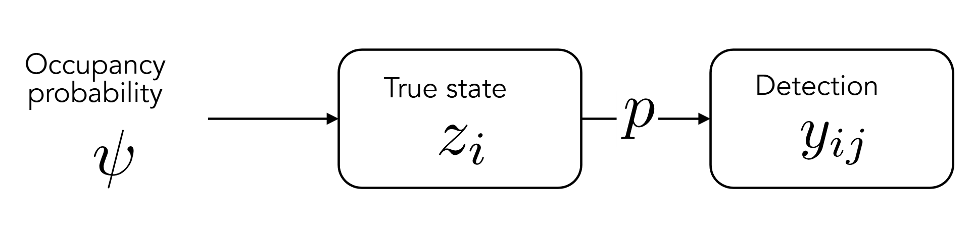
For site \(i\) and visit \(j\): \[ y_{ij} \sim Bern(z_i~p) \] \[ z_i \sim Bern(\psi) \]
Simulate occupancy models in R
Get estimates
Get estimates on the natural scale:
Backtransformed linear combination(s) of Detection estimate(s)

 Estimate     SE LinComb (Intercept)
    0.349 0.0419  -0.623           1

Transformation: logistic
Backtransformed linear combination(s) of Occupancy estimate(s)

 Estimate     SE LinComb (Intercept)
    0.737 0.0788    1.03           1

Transformation: logistic 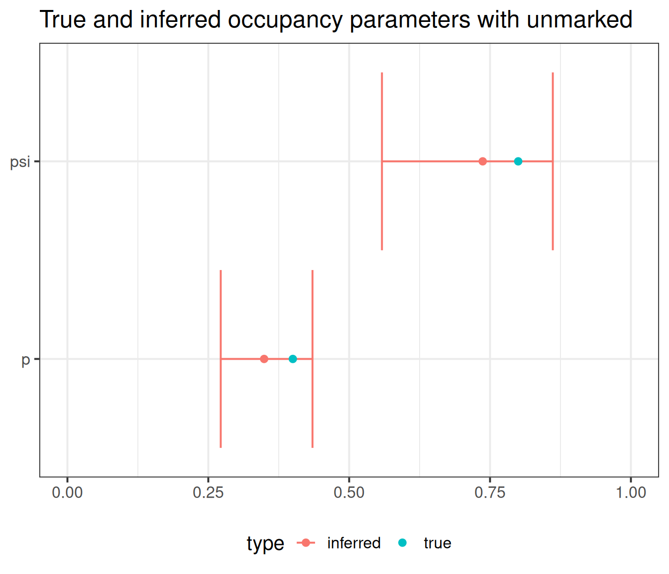
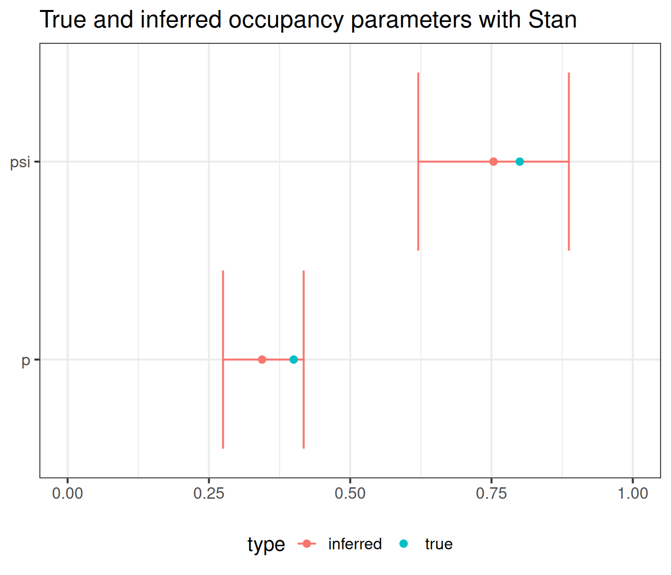
Get estimates
Get parameter estimates:
# A tibble: 5 × 10
  variable      mean   median     sd    mad       q5      q95  rhat ess_bulk
  <chr>        <dbl>    <dbl>  <dbl>  <dbl>    <dbl>    <dbl> <dbl>    <dbl>
1 lp__      -115.    -114.    1.02   0.801  -117.    -114.     1.01     882.
2 psi_logit    1.18     1.11  0.484  0.440     0.491    2.06   1.00    1011.
3 p_logit     -0.651   -0.649 0.190  0.183    -0.970   -0.332  1.00     771.
4 p            0.344    0.343 0.0427 0.0409    0.275    0.418  1.00     771.
5 psi          0.754    0.753 0.0795 0.0808    0.620    0.887  1.00    1011.
# ℹ 1 more variable: ess_tail <dbl>